Data Mining as an Extension of
|
|
What is and isn’t data mining
Data mining is a cluster of techniques, including classification trees, neural networks, and K-mean clustering, which has been employed in the field Business Intelligence (BI) for years (Han & Kamber, 2006). According to Larose (2005), data mining is the process of automatically extracting useful information and relationships from immense quantities of data. Data mining does not start from a strong pre-conception, a specific question, or a narrow hypothesis, rather it aims to detect patterns that are already present in the data and these patterns should be considered relevant to the data miner. Of a similar vein, Luan (2002) views data mining as an extension of Exploratory Data Analysis (EDA). In short, data mining possesses the following characteristics: (a) the utilization of automated algorithms, (b) the utilization of large quantities of data, and (c) an emphasis of exploration and pattern recognition instead of confirming or disconfirming a pre-defined hypothesis or model. In addition, typical data mining techniques include cross-validation, which is considered a form of resampling (Yu, 2003, 2007). The major goal of cross-validation is to avoid overfitting, which is a common problem when modelers try to account for every structure in one data set. As a remedy, cross-validation double-checks whether the alleged fitness is too good to be true (Larose, 2005). Hence, data mining can be viewed as an extension of both EDA and resampling.
It is a common perception that analysis utilizing a large amount of data can be called data mining. Actually, some studies using the term “data mining” did not go beyond classical logistic and linear regression analyses (e.g. Campbell & Collins, 2006). Data mining is a collection of procedures whose underlying logic is substantively different from that of conventional procedures. In this study three data mining tools, namely, classification tree, neural networks, and multivariate adaptive regression splines (MARS) will be introduced and you will clearly see that how their logic is different from traditional techniques.
Differences between DM and conventional procedures
Several researchers conducted comparisons between traditional parametric procedures and data mining techniques (Baker & Richards, 1999; Beck, King, & Zeng, 2000, 2004; Fedenczuk, 2002; Gonzalez & DesJardins, 2002; Naik & Ragothaman, 2004), and also within the domain of data mining procedures (Francis, 2003; Rosella, 2007; Safer, 2003;). It is not surprising to learn that on some occasions one technique outperforms others in terms of prediction accuracy while in a different setting another technique seems to be the best. Using data mining is more appropriate to the study of retention and other forms of institutional analysis than its classical counterpart. First, using such large sample sizes as are found in institutional research will cause the statistical power for any parametric procedures to be 100%. On the contrary, data mining techniques are specifically designed for large data sets. Second, conventional procedures usually require parametric assumptions, such as multivariate normality and homogeneity of variance. In institutional data sets, the distribution of some variables, such as high school GPA and SAT, are highly skewed. Applicants whose academic performance falls below the requirements are typically rejected by the university. Thus, the parametric assumptions are often violated in these data structures. However, data mining procedures are non-parametric and do not rely on these assumptions. Third, institutional research data elements represent multiple data types, including discrete, ordinal, and interval scales. Traditional techniques, such as logistic or linear regression or discriminant function analysis, cannot handle this kind of complexity of data types in one single analysis unless tremendous data transformation, such as converting categorical variables to dummy codes, is used (Streifer & Shumann, 2005).
More importantly, most conventional procedures do not adequately address two important issues, namely, generalization across samples and under-determination of theory by evidence (Kieseppa, 2001). It is very common that in one sample a set of best predictors was yielded from regression analysis, but in another sample a different set of best predictors was found (Thompson, 1995). In other words, this kind of model can provide a post hoc explanation for an existing sample (in-sample forecasting), but cannot be useful in out-of-sample forecasting. This occurs when a specific model is overfitted to a specific data set and thus it weakens generalizability of the conclusion. Further, even if a researcher found the so-called best fit model, there may be numerous possible models to fit the same data.
Nevertheless, data mining procedures have built-in features that can counteract the preceding problems. In most data mining procedures cross-validation is employed based on the premise that exploratory modeling using the training data set inevitably tends to over-fit the data. Hence, in the subsequent modeling using the testing data set, the overfitted model will be revised in order to enhance its generalizability. Specifically, the philosophy of MARS is built upon balancing the overfitted local models and the underfitted global model. MARS partitions the space of input cases into many regions in which local models fitting with cubic splines are generated. Later MARS adapts itself across the input space to generate the best global model.
To remediate the problem of under-determination of theory by data, neural networks exhaust different models by the genetic algorithm, which begins by randomly generating pools of equations. These initial randomly generated equations are estimated to the training data set and prediction accuracy of the outcome measure is assessed using the test set to identify a family of the fittest models. Next, these equations are hybridized or randomly recombined to create the next generation of equations. Parameters from the surviving population of equations may be combined or excluded to form new equations as if they were genetic traits inherited from their “parents.” This process continues until no further improvement in predicting the outcome measure of the test set can be achieved (Baker & Richards, 1999).
Further, there are significant differences between the conventional parametric procedures and data mining in terms of their epistemology. Besides integrating resampling as mentioned before, the philosophy of data mining is in alignment with exploratory data analysis (EDA) (Luan, 2002; Streifer & schumann, 2005). Instead of testing a formulated hypothesis with a pre-specific Alpha level and rejection region, typically data mining research questions begin with “what is” by visualizing data sets and getting simple summaries of them. With low-dimensional data sets, EDA is very useful for data summary and visualization. However, as the dimensionality increases, its performance to visualize inter-dimensional relations decreases. On the other hand, data mining tools are specifically made for multiple-dimensional data sets. Like EDA, data mining is data-driven. The strength of data mining tools, such as neural networks, do not require prior knowledge of the functional relationship between the dependent and independent variables. Rather, neural networks learn from initial examples and gradually recognize the data pattern (Beck, King, & Zeng, 2004; Gonzalez & DesJardins, 2002). But unlike EDA that passes the initial finding to confirmatory data analysis (CDA), data mining tools, with the use of resampling, can go beyond the initial sample to validate the finding (Cuzzocrea, Saccardi, Lux, Porta, & Benatti, 1997). A brief introduction to classification tree, neural networks, and MARS techniques are provided.
Classification trees
Classification trees, developed by Breiman et al. (1984), aim to find which independent variable(s) can make successively a decisive spilt of the data by dividing the original group of data into pairs of subgroups in the dependent variable. In programming terminology, a classification tree can be viewed as a set of “nested-if” logical statements. Breiman et al. used this example for illustrating nested-if logic: When heart attack patients are admitted to a hospital, physiological measures, including heart rate, blood pressure, and background information of the patient, such as personal medical history and family medical history, are usually obtained. Subsequently, patients can be tracked to see if they survive the heart attack for a period of time. In order to determine which piece of information is most relevant to the survival of patients, Breiman et al. developed a three-question decision tree. The three questions are: What is the patient's minimum systolic blood pressure over the initial 24 hour period? What is his/her age? Does he/she display sinus tachycardia? The answers to these three questions can help the doctor to make a quick decision: “If the patient's minimum systolic blood pressure over the initial 24 hour period is greater than 91, then if the patient's age is over 62.5 years, then if the patient displays sinus tachycardia, then and only then the patient is predicted not to survive for at least 30 days.” These nested-if decisions can be translated into a leaf report showing the conditional probability of each combination of variables, and also into a graphical form as a tree structure. A classification tree can be somewhat complicated due to the size of the tree. But, graphical procedures can help to simplify interpretation for the final decision making. Because classification trees can provide guidelines for decision-making, they are also known as decision trees. It is important to note that data mining focuses on pattern recognition, hence no probabilistic inferences and Type I error are involved. Also, unlike regression that returns a subset of variables, classification trees can rank order the factors that affect the retention rate.
Figure 1. Example of classification tree
In data mining processes, including modeling with classification trees and MARS, the model should be deliberately overfit and then scale back to the optimal point. If a model is built from a forward stepping and a stopping rule, the researcher will miss the opportunities of seeing what might be possible and better ahead. Thus, the model must be overfit and then the redundant elements are pruned (Quinlan, 1993; Salford Systems, 2002). Figure 1 is a typical example of a classification tree.
Node splitting in a classification tree is based upon the entropy algorithm, in which the LogWorth statistics is used. To be specific, a decision tree is built in a top-down fashion by examining which variable can best create subgroups that contain instances with similar values (pure or homogeneous). "Entropy" literally means "degradation to disorder" or "chaos." If the sample is completely homogeneous, it is in order and thus the entropy is zero. The ideal situation is like the following: when X = 1, all subjects are in Stage 1. But it is impossible to obtain perfect homogeneity, of course. It is expected to see there is some degree of heterogeneity in each node. If the entropy algorithm determines that a node cannot be further partitioned into fairly homogeneous subsets, that node is closed.
LogWorth is calculated as: -log10(p-value) where the p-value is calculated by taking into account the number of different ways splits can occur. This p value is associated with the difference in the error sum of squares (SS) due to the split. The splits can also be determined by maximizing a LogWorth statistic, which is related to the likelihood ratio chi-square statistic, known as "G^2". As the logworth increases, the p value is smaller, meaning that the Chi-square value for the model is larger. In other words, a bigger logworth means a spilt on the variable can better isolate pure homogeneous subgroups (less entropy or chaos) (SAS Institute, 2011).
To retrospectively examine how accurate the prediction is, receiver operating characteristic (ROC) curve should be used. In any predictive modelling there would be four possible outcomes: true positive (TP), false positive (FP), false negative (FN), and true negative (TN). ROC curves show the points of sensitivity vs. 1 - specificity corresponding to different particular decision thresholds (splits). Sensitivity is obtained by TP/(TP+FN) whereas specificity is obtained by TN/(FP+TN). The ideal prediction outcomes are 100% sensitivity (all true positives are found) and 100% specificity (no false positives are found). It hardly happens in reality, of course. Practically speaking, a good classification tree should depict a ROC curve leaning towards the upper left of the graph, which implies approximation to the ideal. Figure 2 is an example of ROC. In the graph the "area" stands for the area under the ROC curve (AUC), which shows discrimination or classification accuracy. In other words, it tells us how good the model can discriminate between students who tend to stay in the university and those who tend to drop out.
Figure 2. Example of ROC
Table 1 shows the criteria for interpreting AUC values (Homsmer & Lemeshow, 2000). In this case, 0.5544 is just slightly better than pure chance (0.5).
Table 1. Criteria of AUC
AUC value
Interpretation
Between 0.5 and 0.69
No discrimination (you can flip a coin to obtain .5)
Between 0.7 and 0.79
Acceptable
Between 0.8 and 0.89 Excellent
0.9 or above
Outstanding
MARS
MARS is a data mining technique (Friedman, 1991; Hastie, Tishirani, & Friedman, 2001) for solving regression-type problems. Originally, it was made to predict the values of a continuous dependent variable from a set of independent or predictor variables. Later it was adapted into modeling with a binary variable as the outcome variable. Like EDA, MARS is a nonparametric procedure, and thus no functional relationship between the dependent and independent variables is assumed prior to the analysis. MARS accepts the premise that most relevant variables affect the outcome in a complex way. Thus, MARS “learns” about the inter-relationship from a set of coefficients and basis functions in a data-driven fashion. MARS adopts a “divide and conquer” strategy by partitioning the input space into regions, in which a local model is built with its own regression equation. When MARS considers whether to add a variable, it simultaneously searches for appropriate break points, namely, knots. In this initial stage MARS tests variables and potential knots, resulting in an overfit model. In the next stage MARS eliminates redundant variables that do not hold themselves under rigorous testing based upon the criterion of lowest generalized mean square errors in generalized cross validation (GCV). Because a global model tends to be biased but have low variance while local models are more likely to have less bias but suffer from high variance, the MARS approach could be conceptualized as a way to balance between bias and variance.
The strategy of building a global model from local models makes MARS suitable for problems with a larger number of variables and thus remediates “the curse of dimensionality.” Hence, a global model can be built by achieving an optimal point by balancing overfit and unfit models, even if the relationship between the predictors and the dependent variables is non-monotone and difficult to approximate with parametric models.
Unlike conventional statistical procedures that either omit missing values or employ data imputation, MARS generates new variables when encountering variables that have missing values. The missing value indicators are used to develop surrogate sub-models when some needed data are missing.
Neural networks
Neural networks, as the name implies, try to mimic interconnected neurons in animal brains in order to make the algorithm capable of complex learning for extracting patterns and detecting trends (Kuan, 1994; McMenamin, 1997). It is built upon the premise that real world data structures are complex, and thus it necessitates complex learning systems. A trained neural network can be viewed as an “expert” in the category of information it has been given to analyze. This expert system can provide projections given new solutions to a problem and answer "what if" questions. A typical neural network is composed of three types of layers, namely, the input layer, hidden layer, and output layer. It is important to note that there are three types of layers, not three layers, in the network. There may be more than one hidden layer and it depends on how complex the researcher wants the model to be. The input layer contains the input data; the output layer is the result whereas the hidden layer performs data transformation and manipulation. Because the input and the output are mediated by the hidden layer, neural networks are commonly seen as a “black box.”
The network is completely connected in the sense that each node in the layer is connected to each node in the next layer. Each connection has a weight and at the initial stage and these weights are just randomly assigned. A common technique in neural networks to fit a model is called back propagation. During the process of back propagation, the residuals between the predicated and the actual errors in the initial model are fed back to the network. In this sense, back propagation is in a similar vein to residual analysis in EDA (Behrens & Yu, 2003). Since the network performs problem-solving through learning by examples, its operation can be unpredictable. Thus, this iterative loop continues one layer at a time until the errors are minimized. As discussed before, neural networks address the problem of under-determination of theory by evidence with use of multiple paths for model construction. Each path-searching process is called a “tour” and the desired result is that only one best model emerges out of many tours. Like other data mining techniques, neural networks also incorporate cross-validation to avoid capitalization on chance alone in one single sample. Figure 3 is an example of neural network output
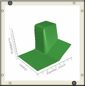
Figure 3. Example of NN
Concluding remarks
This write-up introduces several popular exploratory data mining tools, including recursive classification tree, MARS, and neural networks. It is important to point out that data mining and conventional statistical procedures are not mutually exclusive. Many data miners, such as SAS Enterprise Miner (SAS Institute, 2010a), JMP (SAS Institute, 2010b), IBM SPSS modeler (SPSS Inc., 2017), and Spotfire Miner (TIBCO, 2009) allow researchers to run data mining and conventional procedures side by side. The results from different procedures could be compared against each other using classification agreement and lift charts. This comparison could help researchers to select the best model. To view how the comparison works, please view this demo of using Spotfire Miner. It takes about 3 -7 minutes to download the AVI movie. Video streaming will be introduced in the near future.
References
Behrens, J. T. & Yu, C. H. (2003). Exploratory data analysis. In J. A. Schinka & W. F. Velicer, (Eds.). Handbook of psychology Volume 2: Research methods in Psychology (pp. 33-64). New Jersey: John Wiley & Sons, Inc.
Baker, B. D., & Richards, C. E. (1999). A comparison of conventional linear regression methods and neural networks for forecasting educational spending. Economics of Education Review, 18, 405-415.
Beck, N., King, G., & Zeng, L. (2000). Improving quantitative studies of international conflict: A conjecture. American Political Science review, 94, 21-35.
Beck, N., King, G., & Zeng, L. (2004). Theory and evidence in international conflict: A response to de Marchi, Gelpi, and Grynaviski. American Political Science review, 98, 379-389.
Breiman, L., Friedman, J.H., Olshen, R.A., & Stone, C.J. (1984). Classification and regression trees. Monterey, CA: Wadsworth International Group.
Campbell, J., & Collins, B. (2006 October). Mining student data to support early intervention initiatives. Paper presented at Academic Impressions Web Conference.
Cuzzocrea, G., Saccardi, A., Lux, G., Porta, E., Benatti, A. (1997 March). How many good fishes are there in our Net? Neural networks as a data analysis tool in CDE-Mondadori’s data warehouse. Paper presented at the Annual meeting of SAS User Group International, San Diego, CA.
Fedenczuk, L. (2002 April). To neural or not to neural? This is the question. Paper presented at the Annual Meeting of SAS User Group International, Orlando, FL.
Francis, L. (2003). Martian chronicles: Is MARS better than neural networks? Retrieved May 2007 from http://www.salfordsystems.com/doc/03wf027.pdf
Friedman, J. (1991). Multivariate adaptive regression splines. Annals of Statistics, 19, 1-67.
Gonzalez, J., & DesJardins, S. (2002). Artificial neural networks: A new approach to predicting application behavior. Research in Higher Education, 43, 235-258.
Han, J., & Kamber, M. (2006). Data mining: Concepts and techniques (2nd ed.). Boston, MA: Elsevier.
Hastie, T., Tishirani, R., & Friedman, J. (2001). The elements of statistical learning: Data mining, inference, and prediction. New York, NY: Springer.
Hosmer, D. W., & Lemeshow, S.. (2000). Applied logistic regression. New York, NY: John Wiley & Sons.
Kieseppa, I. A. (2001). Statistical model selection criteria and the philosophical problem of underdetermination. British Journal for the Philosophy of Science, 52, 761–794.
Kuan, C., & White, H. (1994). Artificial neural networks: An econometric perspective. Econometric reviews, 13, 1-91.
Larose, Daniel (2005). Discovering knowledge in data: An introduction to data mining. NJ: Wiley-Interscience.
McMenamin, J. S. (1997). A primer on neural networks for forecasting. Journal of Business Forecasting, 16, 17–22.
Naik, B., & Ragothaman, S. (2004). Using neural networks to predict MBA student success. College Student Journal, 38, 143-149.
Quinlan, J. R. (1993). C4.5 programs for machine learning. San Francisco, CA: Morgan Kaufmann.
Rosella, Inc. (2007). Decision tree classification software. Retrieved January 29, 2007 from http://www.roselladb.com/decision-tree-classification.htm
Safer, A. M. (2003). A comparison of two data mining techniques to predict abnormal stock market returns. Intelligent Data Analysis, 7, 3-13.
Salford Systems. (2002). MARS. [Computer software and manual]. San Diego, CA: The Author.
Salford Systems. (2005). CART. [Computer software and manual]. San Diego, CA: The Author.
SAS Institute. (2010a). Enterprise Miner [Computer software and manual]. Cary, NC: Author.
SAS Institute. (2010b). JMP [Computer software and manual]. Cary, NC: Author.
SAS Institute. (2011). Applied analytics Using SAS Enterprise Miner. Cary, NC: Author.
SPSS, Inc. (2017). IBM SPSS Modeler [Computer software and manual]. Chicago, IL: Author.
Streifer, P. A., & Schumann, J. A. (2005). Using data mining to identify actionable information: breaking new ground in data-driven decision making. Journal of Education for Students Placed at Risk, 10, 281-293.
TIBCO (2009). Spotfire Miner [Computer software and manual]. Palo Alto, CA: The Author.
Thompson, B. (1995). Stepwise regression and stepwise discriminant analysis need not apply here: A guidelines editorial. Educational and Psychological Measurement, 55, 4, 525-534.
Yu, C. H. (2003). Resampling methods: Concepts, applications, and justification. Practical Assessment Research and Evaluation, 8(19) Retrieved from http://pareonline.net/getvn.asp?v=8&n=19
Yu, C. H. (2007). Resampling: A conceptual and procedural introduction. In Jason Osborne (Ed.). Best practices in quantitative methods (pp. 283-298). Thousand Oaks, CA: Sage Publications.
Acknowledgments: Special thanks to Mr. Charles Kaprolet and Ms. Lori Long for their editing of this article.
Related article: Merits and characteristics of text mining
Navigation
Table of
Contents
Main
Table of Contents
Simplified
Navigation
Search
Engine