Gabriel Biplot for
Principal Component Analysis and
Factor Analysis

The objective of this article is to explain the concepts of eigenvector, eigenvalue, variable space, and subject space, as well as the application of these concepts to factor analysis and regression analysis. Gabriel Biplot (Gabriel, 1981; Jacoby, 1998) in SAS/JMP will be used as an example.

You may come across such terms as eigenvalue and eigenvector in factor analysis and principal component analysis (PCA). Although factor analysis and PCA are two different procedures, some researchers found that the procedures yield almost identical results on many occasions. PROC FACTOR in SAS even makes PCA as the default method. And so is SPSS (see the figure on the right).

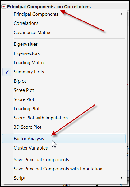
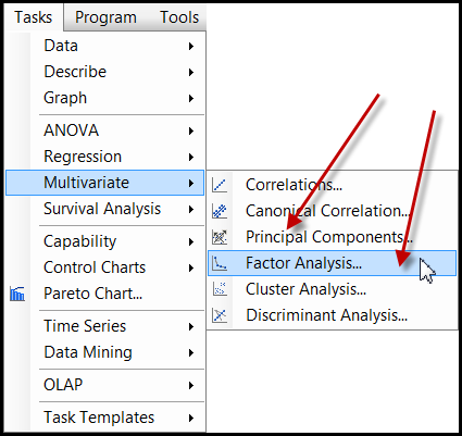
In JMP you can request factor analysis after running PCA or specify maximum likelihood (ML) as the estimation method. Alternatively, you can request factor analysis from Consumer Research. In other words, in JMP factor analysis can be directly accessed without going through PCA. In SAS both options are shown in the Tasks menu.

However, PCA is for data reduction whereas factor analysis is for identify latent constructs. Additionally, the former takes all variances into account while the latter extract shared variances. Therefore, some authors emphasize the demarcation (Bandolas & Boehm-Kaufman, 2009). It is beyond the scope of this brief write-up to discuss the distinction between PCA and factor analysis. In this brief write-up, the focus is on explaining "eigenvalue" and "eigenvector" in layperson terms.

What are "eigenvalue" and "eigenvector"? Are these terms from an alien language?  No, they are from earth. We deal with numbers every day. A mathematical object with a numeric value is called a scalar. A mathematical object that has both a numeric value and a direction is called a vector. If I just tell you to drive 10 miles to reach my home, this instruction is definitely useless. I must say something like, "From Tempe drive 10 miles West to Phoenix." This example shows how essential it is to have both quantitative and directional information.

If you are familiar with computing networking, you may know that the Distance Vector Protocol is used for a network router to determine which path is the best way to transmit data. Again, the router must know two things: Distance (how far is the destination from the source?) and Vector (To what direction should the data travel?)

Another example can be found in computer graphics. There is a form of computer graphics called vector-based graphics, which is used in Adobe Illustrator, Macromedia Flash, and Paint Shop Pro. In vector-based graphics, the image is defined by the relationships among vectors instead of the composition of pixels. For example, to construct a shape, the software stores the information like "Start from point A, draw a straight line at 45 degrees, stop at 10 units, draw another line at 35 degrees..." In short, the scalars and vectors of vector-based graphics define the characteristics of an image.

In the context of statistical analysis, vectors help us to understand the relationships among variables. The word eigen, coined by Hilbert in 1904, is a German word, which literally means "own", "peculiar", or "individual." The most common English translation is characteristic. An Eigenvalue has a numeric property while an eigenvector has a directional property. These properties together define the characteristics of a variable. The original German word emphasizes the unique nature of a specific transformation in Eigenvalues. Eigenvalues and eigenvectors are mathematical objects in which inputs are largely unaffected by a mathematical transformation.

Data as matrix

To understand how eigenvalue and eigenvector work, the data should be considered as a matrix, in which the column vector represents the subject space while the row vector represents the variable space. The function of eigenvalue can be conceptualized as the characteristic function of the data matrix. For convenience, I will use an example with only two variables and two subjects:

	GRE-Verbal	GRE-Quant
David	550	575
Sandra	600	580

The above data can be viewed as a matrix as the following.

550 575
600 580
The columns of the above matrix denote the subject space, which are {550, 600} and {575, 580}. The subject space tells you that between the subjects, David and Sandra, how GRE-Verbal and GRE-Quantitative scores are distributed, respectively. The rows reflect the variable space, which are {550, 575} and {600,580}. The variable space indicates that across the variables GRE-V and GRE-Q, how the scores of the subjects are distributed, respectively.

Variable space

In a scatterplot we deal with the variable space. In the plot on the right, GRE-V lies on the X-axis whereas GRE-Q is on the Y-axis. The data points are the scores of David and Sandra. In a two data-point case, the regression line is perfect, of course.

Subject space

The graph on the right is a plot of subject space. In this graph the X axis and Y axis represent Sandra and David. In GRE-V David scores 550 and Sandra scores 600. A vector is drawn from 0 to the point where Sandra's and David's scores meet (the scale of the graph is not of the right proportion. Actually it starts from 500 rather than 0 in order to make other portions of the graph visible). The vector for GRE-Q is constructed in the same manner.

In reality, a research project always involves more than two variables and two subjects. In a multi-dimensional hyperspace, the vectors in the subject space can be combined to form an eigenvector, which depicts the Eigenvalue. The longer the length of the eigenvector is, the higher the Eigenvalue is and the more variance it can explain. When subject space and variable space are combined, we call it the hyperspace.

Promixity of vectors: Correlation between variables

Eigenvectors and Eigenvalues can be used in regression diagnosis and principal component analysis. In a regression model the independent variables should not be too closely correlated, otherwise the variance explained (R²) will be inflated due to redundant information. This problem is commonly known as "collinearity," which means that the "independent" variables are linearly dependent on each other. In this case the higher variation explained is just due to duplicated information.
 

For example, assume that you are questioning whether you should use GRE-V and GRE-Q together to predict GPA. In a two-subject case, you can examine the relationship between GRE-Q and GRE-V by looking at the proximity of two vectors. When the angle between two vectors is large, both GRE-Q and GRE-V can be retained in the model. But if two vectors exactly overlap or almost overlap each other, then the regression model must be refined.

As mentioned before, the size of Eigenvalues can also tell us the strength of association between the variables (variance explained). When computing a regression model in the variable space, you can use Variation Inflation Factor (VIF) to detect the presence of collinearity. Eigenvalue can be conceptualized as a subject space equivalence to VIF.

Factor analysis: Maximizing Eigenvalues

In regression analysis a high Eigenvalue is bad. On the contrary, a high Eigenvalue is good when the researcher is intended to collapse several variables into a few principal components or factors. This procedure is commonly known as factor analysis or principal component analysis (As mentioned in the beginning, they are not the same things. But explaining their difference is out of the scope of this write-up). For example, GRE-Q, GRE-V, GMAT, and MAT may be combined as a factor named "public exam scores." Motivation and self-efficacy may be grouped as "psychological factor."

Because many people are familiar with regression analysis, in the following regression is used as a metaphor to illustrate the concept.
 

We usually depict regression in the variable space. In the variable space the data points are people. The purpose is to fit the regression line with the people. In other words, we want the regression line passes through as many people as possible with the least distance between the regression line and the data points. This criterion is called least square, which is the sum of square of the residuals.

In factor analysis and principal component analysis, we jump from variable space into subject space. In the subject space we fit the factor with the variables. The fit is based upon factor loading--variable-factor correlation. The sum of square of factor loadings is Eigenvalue. According to Kaiser's rule, we should retain the factor which has an Eigenvalue of one or above.

The following table summarizes the two spaces:
 

	Variable space	Subject space
Graphical representation	The axes are variables whereas the data points are people.	The axes are people whereas the data points are variables.
Reduction	The purpose of regression analysis is to reduce a large number of people's responses into a small manageable number of trends called regression lines.	The purpose of factor analysis is to reduce a large number of variables into a small manageable number of factors which are represented by Eigenvectors.
Fit	This reduction of people's responses is essentially to make the scattered data form a meaningful pattern. To find the pattern in variable space we "fit" the regression line to the people's responses. In statistical jargon we call it the best fit.	In subject space we look for the fit between the variables and the factors. We want each variable to "load" into the factor most related to it. In statistical jargon we call this factor loading.
Criterion	In regression we sum the squares of residuals and make the best fit based on the least square. These are the criteria used to make the reduction and the fit.	In factor analysis we sum the squares of factor loadings to get the Eigenvalue. The size of the Eigenvalues determines how many factors are "extracted" from the variables.
Structure	In regression we want that the regression line passes through as many points as possible.	In factor analysis the Eigenvalue is geometrically expressed in the eigenvector. We want the eigenvector passes through as many points as possible. In statistical jargon we call this simple structure, which will be explained later.
Equation	In regression the relationship between the outcome variable and the predictor variables can be expressed in a weighted linear combination such as Y = a + b1X1 + b2X2 + e.	In factor analysis the relationship between the latent variable (factor) and the observed variables can also be expressed in a weighted linear combination such as Y = b1X1 + b2X2 except that there is no intercept in the equation.

Factor rotation:
Positive Manifold and Simple Structure

After determining how many factors can be extracted from the variables, we should find out which variables are loaded into which factors. There are two major criteria, namely, positive manifold and simple structure. It is very rare that the variables are loaded properly into different factors at the first time. The researcher must rotate the factors in order to meet the preceding criteria.
 

Positive manifold: The data may turn out having large positive and negative loadings. If you know that your factors are bipolar e.g. introvert personality and extrovert personality, it is acceptable. If your factors are measuring quantitative intelligence and verbal intelligence, they may be lowly correlated but should not go to opposite directions. In other words, students who score very good in math may not have equal performance in English, but their English scores should not be extremely poor. In this case, you had better rotate the factors to get as many positive loadings as possible.

Simple structure: Simple structure suggests that any one variable should be highly related to only one factor and most of the loadings on any one factor should be small. If some variables have high loadings into several factors, the researcher must rotate the factors. For instance, in the following case most variables are loaded into Factor A, and variable 3 and 5 have high loadings in both Factor A and B.
 

	Factor A	Factor B
Variable 1	.75	.32
Variable 2	.79	.21
Variable 3	.64	.67
Variable 4	.10	.50
Variable 5	.55	.57

After rotation the structure should be less messy and simpler. In the following case, variable 1, 3, and 5 are loaded into factor A while variable 2 and 4 are loaded into factor B:
 

	Factor A	Factor B
Variable 1	.63	.39
Variable 2	.49	.66
Variable 3	.77	.27
Variable 4	.03	.70
Variable 5	.75	.33

Gabriel Biplot:
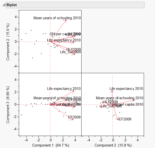
Combining subject space and variable space

Gabriel biplot (Gabriel, 1981), which is available in Vista (top) and JMP (bottom), is a visualization technique for principal component analysis. Biplot simply means a plot of two spaces: the subject and variable spaces. In the example shown by the following figures, the vectors labeled as PC1 (principal component 1), PC2 and PC3 are eigenvectors in the subject space, and the observations in the variable space. The user is allowed to specify the number of components and rotate them in order to visually inspect the relationship between the eigenvectors and the observations.

Biplot in Vista

Biplot in JMP

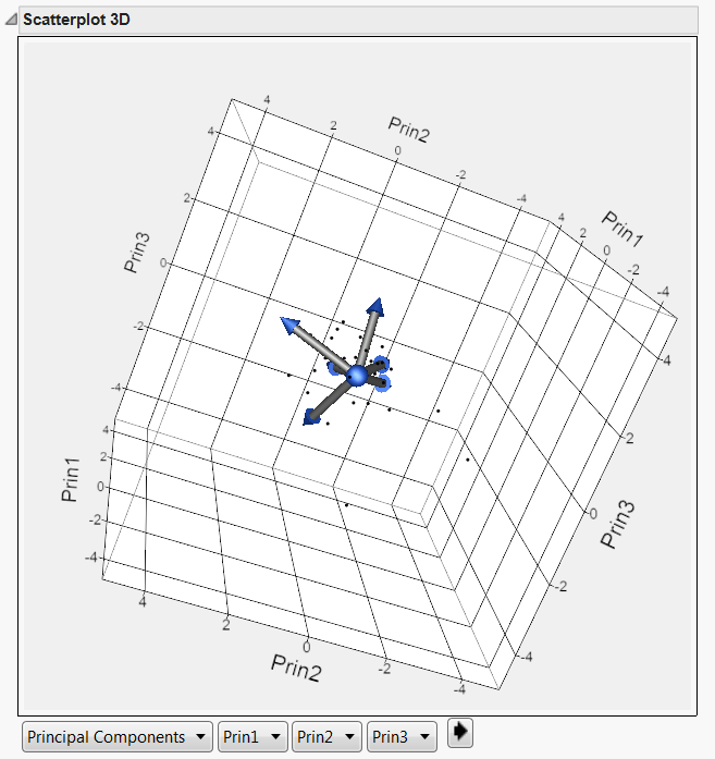
3D score plot in JMP

JMP enables the user to visualize PCA or FA by using both 2D and 3D biplots. In a 2D biplot there are two axes and thus only two principal components can be displayed in a plot. When more than two components or factors are suggested, different panels are needed. In a 3D biplot, three components can be shown simultaneously and the user could rotate the plot to obtain a better view. The axes of the plots are the principal components while the variables are symbolized by rays or vectors radiating from the center. Vectors pointing to the same direction with a small angle between them implies a positive and close relationship between the variables. Due to this characteristic, they could be loaded into the same component. In the above example, it is obvious that Happy Life Year (HLY) and Life Satisfaction could be collapsed as a single construct, but these two variables are far away from Gross National Income (GNI). This concurs with the conventional wisdom that money cannot buy happiness.  

GGEBiplot

Besides SAS/JMP and Vista, several other statistical packages (e.g. Stata, Xlisp-Stat) are also capable of creating a biplot. Nonetheless, by far the most feature-rich biplot is the GGEbiplot invented by Wan and Kang (2003). GGE biplot analysis and GGEbiplot software were originally developed to help plant breeders to understand and explore genotype by environment interactions; nevertheless, its application is readily transportable to psychology, education, and other domains of social sciences. Special features of GGEbiplot include, but are not limited to, data imputation, data transformation.

More importantly, while other biplot graphing programs can handle a 2X2 matrix (subject by variable) only, GGEbiplot goes beyond 2-way tables to 3- and 4-way.

By default, GGEbiplot shows a 2D biplot depicting the location of variables and the first few subjects on the hyperspace (Principal component 1 X Principal component 2; PC1 X PC2).

With just one mouse-click, the user can transform the 2D biplot to a 3D one. The following biplot indicates that these variables (V1-V5) seem to be highly independent due to their diverse directions in the hyperspace, and thus putting them into a single common factor may not be appropriate. You can view an AVI animation of this 3D biplot. 

 

GGEbiplot is downloadable at www.ggebiplot.com

 

References

Bandalos, D. L., & Boehm-Kaufman, M. R. (2009). Four common misconceptions in exploratory factor analysis. In Charles E. Lance & Robert J. Vandenberg (Eds.), Statistical and methodological myths and urban legends: Doctrine, verity and fable in the organizational and social sciences. New York: Routledge.

Gabriel, K. R. (1981). Biplot display of multivariate matrices for inspection of data and diagnosis. In V. Barnett (Ed.) Interpreting multivariate data. London: John Wiley & Sons.

Jacoby, W. G. (1998). Statistical graphics for visualizing multivariate data. Thousand Oaks, CA: Sage Publications.

Yan, W. and Kang, M. S.(2003). GGE Biplot Analysis: A graphical tool for breeders, geneticists, and agronomists. CRC Press. Boca Raton, FL.