Multi-collineartity, Variance Inflation
and Orthogonalization in Regression

Orthogonalization

In spite of its logical independence, we still have to "orthogonalize" the variables to make them mathematically independent. Orthogonality is a state in which the angle between two vectors is 90 degrees. According to Hacking (1992), orthogonality is not only a pure mathematical concept, but also a cultural concept that carries value judgment:

Normal and orthogonal are synonyms in geometry; normal and ortho- go together as Latin to Greek. Norm/ortho has thereby a great power. On the one hand the words are descriptive. A line may be orthogonal or normal (at right angles to the tangent of a circle, say) or not. That is a description of the line. But the evaluative 'right' lurks in the background of right angles. It is just a fact that an angle is a right angle, but it is also a 'right' angle, a good one. Orthodonists straighten the teeth of children; they make the crooked straight. But they also put the teeth right, make them better. Orthopaedic surgeons straighten bones. Orthopsychiatry is the study of mental disorders chiefly in children. It aims at making the child-normal. The orthodox conform to certain standards, which used to be a good thing (p.163).

In the context of regression, orthogonalization can make a "good" regression model. In subject space, "orthogonalization" can be viewed as a process of subtracting the vector from its projection. In variable space, "orthogonalization" can be explained as a process of finding the residual of the interaction term.

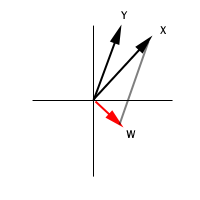
First, let's look at how subtraction works in vector space (subject space). The left panel illustrates how a new vector, W, is made by X - Y. To subtract Y from X, a parallel line of Y is drawn at the end of X. Then a new vector is formed by joining the origin of X,Y and the other end of Y's parallel. In other words, subtraction creates a new vector pointing to a different direction, which is significantly far away from the original vectors! As you see, although X and Y are highly correlated, which is indicated by the small angle between the two vectors, W is uncorrelated to either X or Y. That's why vector subtraction can help to do away with collinearity.

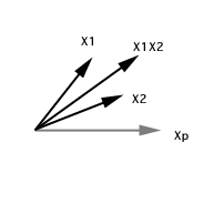
Second, let's talk about projection. Please keep in mind that the following illustration is simplified. The actual orthogonalization is not in the exact same way as described here. Y is omitted from the illustration because in this procedure we care about the regressors only. In the right panel, X1 and X2 are not strongly related. You could tell by the wide angel between the two vectors. However, the product of X1,X2 is strongly associated with either X1 or X2, which is indicated by the proximity between X1 and X1X2, and between X2 and X1X2, respectively (As you notice, the product vector is longer than X1 and X2. In reality the interaction vector is much longer. This will be shown in the next section).

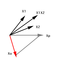
To solve this collinearity problem, the first step is to draw a projection of X1X2 vector. A projection in the subject space is equivalent to the predicted (y-hat) in the variable space. In the right panel, X1X2 is the actual vector and Xp is the predicted vector.

After locating the projection, the next step is to create a new vector (new variable), which is orthogonal (not closely related) to X1 and X2, but is conceptually equivalent to X1X2. By using the subtraction method mentioned above, we can create the new vector Xo. Xo can be viewed as a result of negotiating between what is (X1X2) and what ought to be (Xp). Is this always true in our human world, too? Remember Freudian psychology? A human psychic is composed of id (what is), superego (what ought to be), and ego (the mediator between the two). Before orthogonalization, there exist a threat of collinearity. After orthogonalization, Xo is far away from X1 and X2 and thus collinearity is no longer a threat.

The SAS code for orthogonalizing the interaction term is as the following. This is a partial orthogonalization method suggested by Burrill (1997):

X1X2 = X1*X2

/* this step output the residuals of the interaction term*/

PROC REG DATA=DATA1;
	MODEL X1X2 = X1 X2;
	OUTPUT OUT=DATA2 R=R_X1X2;
/* this step uses the residual as an orthogonalized variable */

PROC REG DATA=DATA2;
	MODEL Y = X1 X2 R_X1X2;

Back

Menu

Next

---

Navigation

Index

Simplified Navigation

Table of Contents

Search Engine

Contact