The problem of too many variables
Stepwise regression
Collinearity happens to many inexperienced researchers. A common
mistake is to put too many regressors into the model. As what I
explained in my example of "fifty ways to improve your grade, "
inevitably many of those independent variables will be too correlated.
In addition, when there are too many variables in a regression model
i.e. the number of parameters to be estimated is larger than the number
of observations, this model is said to be lack of degree of freedom and
thus over-fitting.
The following cases are extreme, but you will get the idea. When there
is one subject only, the regression line can be fitted in any way (left
figure). When there are two observations, the regression line is a
perfect fit (right figure). When things are perfect, they are indeed
imperfect!
One common approach to select a subset of variables from a complex
model is stepwise regression. A stepwise regression is a procedure to
examine the impact of each variable to the model step by step. The
variable that cannot contribute much to the variance explained would be
thrown out. There are several versions of stepwise regression such as forward selection, backward elimination, and stepwise.
Many researchers employed these techniques to determine the order of
predictors by its magnitude of influence on the outcome variable (e.g.
June, 1997; Leigh, 1996).
|
However, the above interpretation is valid if and only if all
predictors are independent (But if you write a dissertation, it doesn't
matter. Follow what your committee advises). Collinear regressors or
regressors with some degree of correlation would return inaccurate
results. Assume that there is a Y outcome variable and four regressors X1-X4. In the left panel X1-X4
are correlated (non-orthogonal). We cannot tell which variable
contributes the most of the variance explained individually. If X1 enters the model first, it seems to contribute the largest amount of variance explained. X2
seems to be less influential because its contribution to the variance
explained has been overlapped by the first variable, and X3 and X4 are even worse.
| 
|
|
Indeed, the more correlated the regressors are, the more their ranked
"importance" depends on the selection order (Bring, 1996). However, we
can interpret the result of step regression as an indication of the
importance of independent variables if all predictors are orthogonal.
In the right panel we have a "clean" model. The individual contribution
to the variance explained by each variable to the model is clearly
seen. Thus, we can assert that X1 and X4 are more influential to the dependent variable than X2 and X3.
|
Maximum R-square, RMSE, and Mallow's Cp
There are other better ways to perform variable selection such as
Maximum R-square, Root Mean Square Error (RMSE), and Mallow's Cp. Max.
R-square is a method of variable selection by examining the best of
n-models based upon the largest variance explanied. The other two are
opposite to max. R-square. RMSE is a measure of the lack of fit while
Mallow's CP is the total square errors, as opposed to the best fit by
max. R-square. Thus, the higher the R-square is, the better the model
is. The lower the RMSQ and Cp are, the better the model is.
For the clarity of illustration, I use only three regressors: X1, X2, X3.
The principle illustrated here can be well-applied to the situation of
many regressors. The following output is based on a hypothetical
dataset:
| Variable |
R-square |
RMSE |
Cp |
| One-variable models |
| X3 |
0.31 |
2.27 |
9.40 |
| X2 |
0.27 |
2.35 |
10.90 |
| X1 |
0.00 |
2.75 |
19.41 |
| Two-variable models |
| X2X3 |
0.60 |
1.81 |
2.70 |
| X1X3 |
0.33 |
2.34 |
11.20 |
| X1X2 |
0.32 |
2.35 |
11.34 |
| Full model |
| X1X2X3 |
0.62 |
1.84 |
4.00 |
At first, each regressor enters the model one by one. In all one-variable models, the best variable is X3 according to the max. R-square criterion (R2=.31).
(Now we temporarily ignore RMSE and Cp). Then, all combinations of
two-variable models are computed. This time the best two predictors are
X2 and X3 (R2=.60). Last, all three variables are used for a full model (R2=.62).
From the one-variable model to the two-variable model, the variance
explained gains a substantive improvement (.60 - .31 = .29). However,
from the two-variable to the full model, the gain is trivial (.62 - .60
= .02).
|
If you cannot follow the above explanation, this figure may help you.
The x-axis represents the number of variables while the y-axis
represents the R-square. It clearly indicates a sharp jump from one to
two. But the curve turns into flat from two to three (see the red
arrow).
|
|
Now, let's examine RMSE and Cp. Interestingly enough, in terms of both
RMSE and Cp, the full model is worse than the two-variable model. The
RMSE of the best two-variable is 1.81 but that of the full model is
1.83 (see the red arrow in the right panel)! The Cp of the best two is
2.70 whereas that of the full model is 4.00 (see the red arrow in the
following figure)!
|
|
|
Nevertheless, although the approaches of maximum
R-square, Root Mean Square Error, and Mallow's Cp are different, the
conclusion is the same: One is too few and three are too many. To
perform a variable selection in SAS, the syntax is "PROC REG; MODEL
Y=X1-X3 /SELECTION=MAXR". To plot Max. R-square, RMSQ, and Cp together,
use NCSS.
|
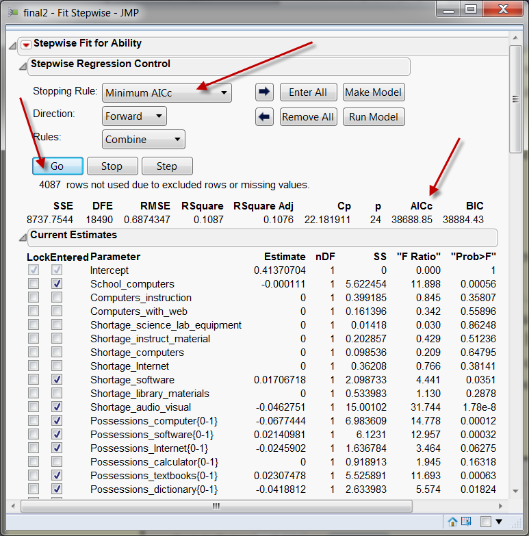
Stepwise regression based on AICc
Although the result of stepwise regression depends on the order of entering
predictors, JMP allows the user to select or deselect
variables in any order. The process is so interactive that the analyst can
easily determine whether certain variables should be kept or dropped. In
addition to Mallows' CP, JMP shows Akaike's information criterion correction (AICc) to
indicate the balance between fitness and simplicity of the model.
The original Akaike's information criterion (AIC) without correction,
developed by Hirotsugu Akaike (1973), is in alignment with Ockham’s
razor: Given all things being equal, the simplest model tends to be the
best one; and simplicity is a function of the number of adjustable
parameters. Thus, a smaller AIC suggests a "better" model.
Specifically, AIC is a fitness index for trading off the complexity of
a model against how well the model fits the data. The general form of
AIC is: AIC = 2k – 2lnL where k is the number of parameters and L is
the likelihood function of the estimated parameters. Increasing the
number of free parameters to be estimated improves the model fitness,
however, the model might be unnecessarily complex. To reach a balance
between fitness and parsimony, AIC not only rewards goodness of fit,
but also includes a penalty that is an increasing function of the
number of estimated parameters. This penalty discourages over-fitting
and complexity. Hence, the “best” model is the one with the lowest AIC
value. Since AIC attempts to find the model that best explains the data
with a minimum of free parameters, it is considered an approach
favoring simplicity. In this sense, AIC is better than R-squared and
adjusted R-squared, which always go up as additional variables enter in
the model. Needless to say, this approach favors complexity. However,
AIC does not necessarily change by adding variables. Rather, it varies
based upon the composition of the predictors and thus it is a better
indicator of the model quality (Faraway, 2005).
AICc is a further step beyond AIC in the sense that AICs imposes a
greater penalty for additional parameters. The formula of AICs is:
AICc = AIC + (2K(K+1)/(n-k-1))
where n = sample size and k = the number of parameters to be estimated.
Burnham and Anderson (2002) recommend replacing AIC with AICc,
especially when the sample size is small and the number of parameters
is large. Actually, AICc converges to AIC as the sample size is getting
larger and larger. Hence, AICc should be used regardless of sample size
and the number of parameters.
Bayesian information criterion (BIC) is similar to AIC, but its penalty is
heavier than that of AIC. However, some authors believe that AIC and AICc are
superior to BIC for a number of reasons. First, AIC and AICc is based on the
principle of information gain. Second, the Bayesian approach requires a prior
input but usually it is debatable. Third, AIC is asymptotically optimal in model
selection in terms of the least squared mean error, but BIC is not
asymptotically optimal (Burnham & Anderson, 2004; Yang, 2005).
JMP provides the users with the options of AICc and BIC for model refinement.
To start running stepwise regression with AICc or BIC, use Fit models and then
choose Stepwise from Personality. These short movie clips show the first and the second
steps of constructing an optimal regression model with AICc (Special
thanks to Michelle Miller for her help in recording the movie clips).
Besides
regression, AIC and BIC are also used in many other statistical
procedures for model selection (e.g. structural equation modeling).
While degree of model fitness is a continuum, the cutoff points of
conventional fitness indices force researchers to make a dichotomous
decision. To rectify the situation, Suzanne and Preston (2015)
suggested replacing arbitrary cutoffs with Akaike Information Criterion
(1973) and Bayesian Information Criterion (BIC). It is important to
emphasize that unlike conventional fitness indices, there is no cutoff
in AIC or BIC. Rather, the researcher explores different alternate
models and then select the best fit based on the least AIC or BIC.
Partial least squares regression
There are other ways to reduce the number of variables such as factor
analysis, principal component analysis and partial least squares. The
philosophy behind these methods is very different from variable
selection methods. In the former group of procedures "redundant"
variables are not excluded. Rather they are retained and combined to
form latent factors. It is believed that a construct should be an "open
concept" that is triangulated by multiple indicators instead of a
single measure (Salvucci, Walter, Conley, Fink, & Saba, 1997). In
this sense, redundancy enhances reliability and yields a better model.
However, factor analysis and principal component analysis do not have
the distinction between dependent and independent variables and thus
may not be applicable to research with the purpose of regression
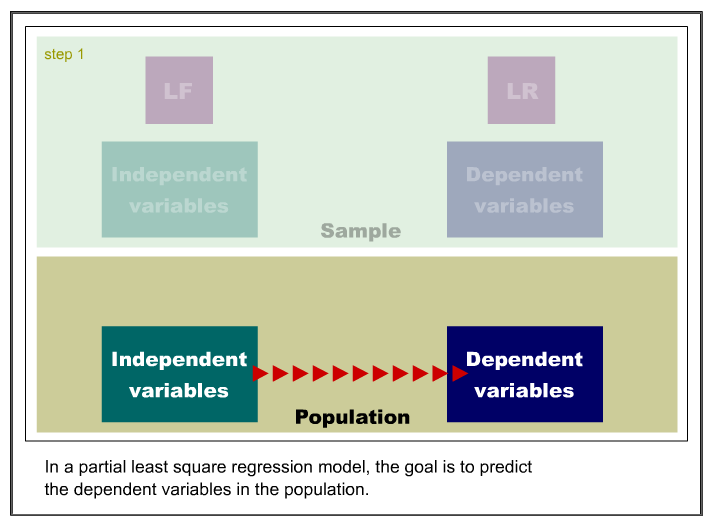
analysis. One way to reduce the number of variables in the context of
regression is to employ the partial least squares (PLS) procedure. PLS
is a method for constructing predictive models when the variables are
too many and highly collinear (Tobias, 1999). Besides collinearity, PLS
is also robust against other data structural problems such as skew
distributions and omission of regressors (Cassel, Westlund, &
Hackl, 1999). It is important to note that in PLS the emphasis is on
prediction rather than explaining the underlying relationships between
the variables. Thus, although some program (e.g. JMP) names the
variables as "factors," indeed they are a-theoretical principal
components.
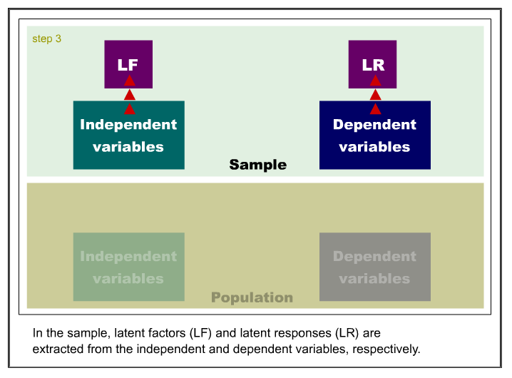
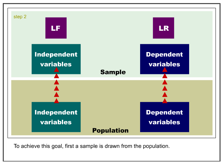
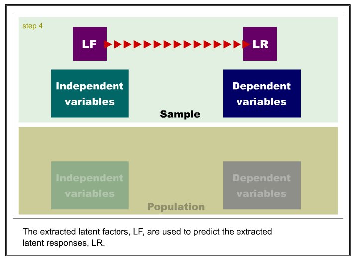
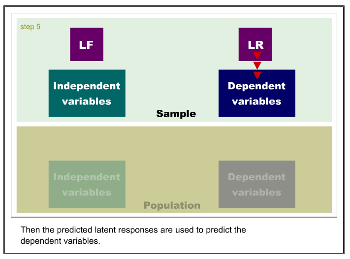
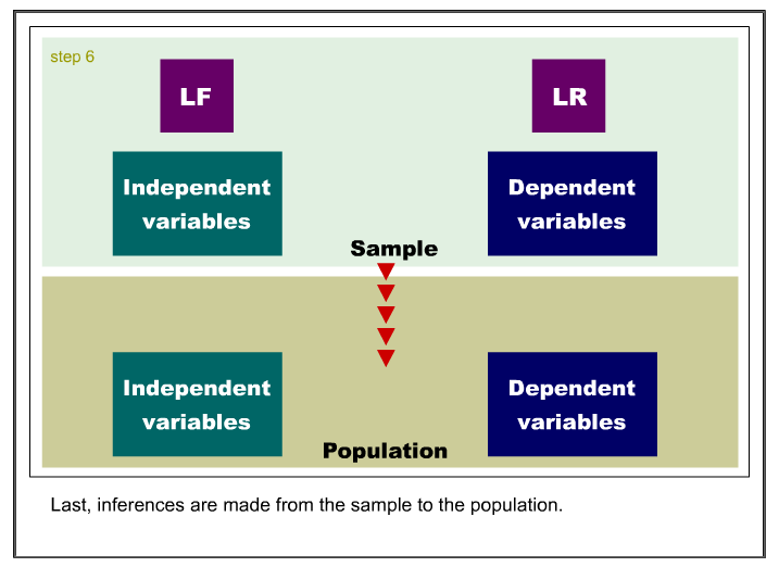
Like principal component analysis, the basic idea of PLS is to extract
several latent factors and responses from a large number of observed
variables. Therefore, the acronym PLS is also taken to mean projection to latent structure.
The following is an example of the SAS code for PLS: PROC PLS; MODEL;
y1-y5 = x1-x100; Note that unlike an ordinary least squares regression,
PLS can accept multiple dependent variables. The output shows the
percent variation accounted for each extracted latent variable:
Number of
latent variables |
Model effects
Current |
Model effects
Total |
DV
Current |
DV
Total |
| 1 |
39.35 |
39.35 |
28.70 |
28.70 |
| 2 |
29.94 |
69.29 |
25.58 |
54.28 |
| 3 |
7.93 |
77.22 |
21.86 |
76.14 |
| 4 |
6.40 |
83.62 |
6.45 |
82.59 |
| 5 |
2.07 |
85.69 |
16.96 |
99.54 |
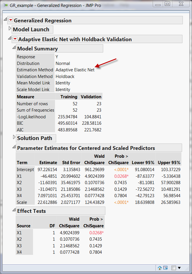
Generalized regression
In
addition to the partial least-square method, a modeler can also use
generalized regression modeling (GRM) as a remedy to the threat of
multicollinearity. GRM, which is available in JMP, offers four
options, namely, maximum likelihood, Lasso, Ridge, and Adaptive Elastic
Net, to perform variable
selection. The basic idea of GRM is very simple: using penalty to avoid
model complexity. Among the preceding four options, adaptive elastic
net is considered the best in most situations because it combines the
strength of Lasso and Ridge. The following is a typical GRM output.
Navigation
Index
Simplified Navigation
Table of Contents
Search Engine
Contact