Illustrating degrees of
freedom
in terms of sample size and
dimensionality
Dr. Chong Ho
(Alex) Yu (2009)
|
"Degree of freedom" (df) is an "intimate stranger" to
statistics students. Every quantitative-based research paper
requires reporting of degrees of freedom associated with the test
results such as "F(df1, df2)," yet very few people understand why
it is essential to do so. Although the concept "degree of freedom"
is taught in introductory statistics classes, many students learn
the literal definition of this term rather than its deeper
meaning. Failure to understand "degrees of freedom" has two side
effects. First, students and inexperienced researchers tend to mis-interpret a "perfect-fitted" model or an "over-fitted" model
as a good model. Second, they have a false sense of security that
df is adequate while n is large. This reflects the problem that
most failed to comprehend that df is a function of both the number
of observations and the number of variables in one's model. Frustration by this
problem among statistical instructors is manifested by the fact
that the issue "how df should be taught" has been recurring in
several statistical-related discussion groups (e.g. edstat-l,
sci.stat.edu, sci.stat.math).
Many elementary statistics textbooks introduce this concept in
terms of the numbers that are "free to vary" (Howell, 1992; Jaccard
& Becker, 1990). Some statistics textbooks just give the df of
various distributions (e.g. Moore & McCabe, 1989; Agresti
& Finlay, 1986). Johnson (1992) simply said that degree of
freedom is the "index number" for identifying which distribution
is used. Some definitions given by statistical instructors can be as
obscured as "a mathematical property of a distribution related to
the number of values in a sample that can be freely specified once
you know something about the sample." (cited in Flatto, 1996)
The preceding explanations cannot clearly show the
purpose of df. Even advanced statistics textbooks do not discuss
the degrees of freedom in detail (e.g. Hays, 1981; Maxwell and Delany,
1986; Winner, 1985). It is not uncommon that many advanced
statistics students and experienced researchers have a vague idea
of the degrees of freedom concept.
There are other approaches taken to present the concept of degree of
freedom. Most of them are mathematical in essence (see Appendix
A). While these mathematical explanations carry some merits, they
may still be difficult to statistical students, especially in social sciences, who generally do not have a
strong mathematical background. In the following section, it is
recommended that df can be explained in terms of sample size and
dimensionality. Both can represent the number of pieces of useful
information.
Df in terms of sample size
Toothaker (1986) explained df as the number of
independent components minus the number of parameters estimated.
This approach is based upon the definition provided by Walker
(1940): the number of observations minus the number of necessary
relations, which is obtainable from these observations (df = n -
r). Although Good (1973) criticized that Walker's approach is not
obvious in the meaning of necessary relations, the number of
necessary relationships is indeed intuitive when there are just a
few variables. The definition of "necessary relationship" is beyond the scope of this article. To avoid confusion, in this
article, it is simply defined as the relationship between a
dependent variable (Y) and each independent variable (X) in the
research.
Please keep in mind that this illustration is simplified for
conceptual clarity. Although Walker regards the preceding equation
as a universal rule, don't think that df = n - r can really be
applied to all situations.
No degree of freedom and effective sample size
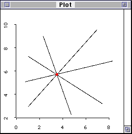
Figure 1 shows that there is one relationship under investigation (r = 1)
when there are two variables. In the scatterplot where there is only one
datum point. The analyst cannot do any estimation of the regression line
because the line can go in any direction, as shown in Figure 1.In other words,
there isn't any useful information.
Figure 1. No degree of freedom with one datum point.
When the degree of freedom is zero (df = n - r = 1 - 1 = 0),
there is no way to affirm or reject the model! In
this sense, the data have no "freedom" to vary and you don't have
any "freedom" to conduct research with this data set. Put it bluntly, one
subject is basically useless, and obviously, df defines the effective
sample size (Eisenhauer, 2008).
Perfect fitting
In order to plot a regression line, you must have at least two
data points as indicated in the following scattergram.
Figure 2. Perfect fit with two data points.
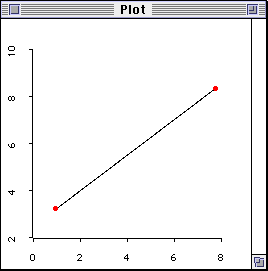
In this case, there is one degree of freedom for estimation (n - 1 = 1,
where n = 2). When there are two data points only, one can always join them
to be a straight regression line and get a perfect correlation (r = 1.00).
Since the slope goes through all data points and there is no residual, it is
considered a "perfect" fit. The word "perfect-fit" can be misleading. Naive
students may regard this as a good sign. Indeed, the opposite is true. When
you marry a perfect man/woman, it may be too good to be true! The so-called
"perfect-fit" results from the lack of useful information. Since the data do
not have much "freedom" to vary and no alternate models could be explored,
the researcher has no "freedom" to further the study. Again, the effective
sample size is defined by df = n -1.
This point is extremely important because very few researchers
are aware that perfect fitting is a sign of serious problems. For
instance, when Mendel conducted research on heredity, the
conclusion was derived from almost "perfect" data. Later R. A.
Fisher questioned that the data are too good to be true. After
re-analyzing the data, Fisher found that the "perfectly-fitted"
data are actually erroneous (Press & Tanur, 2001).
Over-fitting
In addition, when there are too many variables in a regression
model i.e. the number of parameters to be estimated is larger than
the number of observations, this model is said to lacking degrees of freedom and thus is over-fit. To simplify the
illustration, a scenario with three observations and two variables
are presented.
Figure 3. Over-fit with three data points.
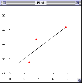
Conceptually speaking, there should be four or more variables,
and three or fewer observations to make a model over-fitting.
Nevertheless, when only three subjects are used to estimate the
strength of association between two variables, the situation is
bad enough. Since there are just a few observations, the residuals
are small and it gives an illustration that the model and the data
fit each other very well. When the sample size is larger and data
points scatter around the plot, the residuals are higher, of
course. In this case, the model tends to be have a lesser degree
of fit. Nevertheless, a less fitted model resulted from more
degrees of freedom carry more merits.
Useful information
Finally, you should see that the degree of freedom is the
number of pieces of useful information.
|
Sample
size
|
Degree(s) of
freedom
|
Amount of
information
|
|
1
|
0
|
no information
|
|
2
|
1
|
not enough information
|
|
3
|
2
|
still not enough
information
|
Falsifiability
 To
further explain why lacking useful information is detrimental to
research, the program ties degrees of freedom to falsifiability.
In the case of "perfect-fitting," the model is "always right." In
"over-fitting," the model tends to be "almost right." Both models
have a low degree of falsifiability. The concept "falsifiability"
was introduced by Karl Popper (1959), a prominent philosopher of
science. According to Popper, the validity of knowledge is tied to
the probability of falsification. Scientific propositions can be
falsified empirically. On the other hand, unscientific claims are
always "right" and cannot be falsified at all. We cannot
conclusively affirm a hypothesis, but we can conclusively negate
it. The more specific a theory is, the higher possibility that the
statement can be negated. For Popper, a scientific method is
"proposing bold hypotheses, and exposing them to the severest
criticism, in order to detect where we have erred." (1974, p.68)
If the theory can stand "the trial of fire," then we can confirm
its validity. When there is no or low degree of freedom, the data
could be fit with any theory and thus the theory is said to be
unfalsifiable. To
further explain why lacking useful information is detrimental to
research, the program ties degrees of freedom to falsifiability.
In the case of "perfect-fitting," the model is "always right." In
"over-fitting," the model tends to be "almost right." Both models
have a low degree of falsifiability. The concept "falsifiability"
was introduced by Karl Popper (1959), a prominent philosopher of
science. According to Popper, the validity of knowledge is tied to
the probability of falsification. Scientific propositions can be
falsified empirically. On the other hand, unscientific claims are
always "right" and cannot be falsified at all. We cannot
conclusively affirm a hypothesis, but we can conclusively negate
it. The more specific a theory is, the higher possibility that the
statement can be negated. For Popper, a scientific method is
"proposing bold hypotheses, and exposing them to the severest
criticism, in order to detect where we have erred." (1974, p.68)
If the theory can stand "the trial of fire," then we can confirm
its validity. When there is no or low degree of freedom, the data
could be fit with any theory and thus the theory is said to be
unfalsifiable.
df in terms of dimensions and
parameters
Now degrees of freedom are illustrated in terms of
dimensionality and parameters. According to I. J. Good, degrees of
freedom can be expressed as
D(K) - D(H),
whereas
D(K) = the dimensionality of a broader hypothesis,
such as a full model in regression
D(H) = the dimensionality of the null hypothesis,
such as a restricted or null model
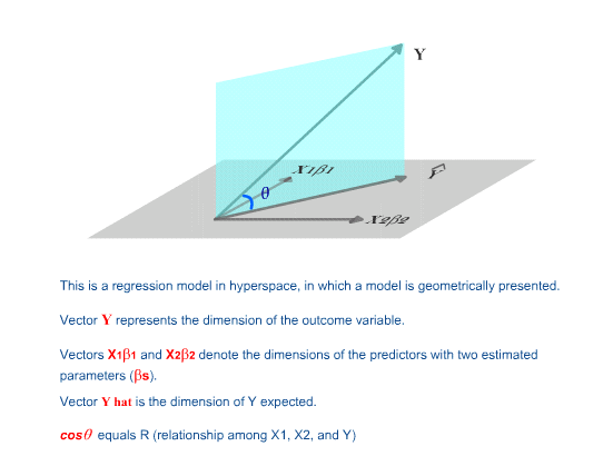
In the following, vectors (variables) in hyperspace are used for
illustration (Saville & Wood, 1991; Wickens, 1995). It is
important to point out that the illustration is only a metaphor to
make comprehension easier. Vectors do not behave literally as
shown.
Figure 4. Vectors in hyperspace.

For the time being, let's ignore the intercept. What is(are)
the degree(s) of freedom when there is one variable (vector) in a
regression model? First, we need to find out the number of
parameter(s) in a one-predictor model. Since only one
predictor is present, there is only one beta weight to be estimated. The
answer is straight-forward. There is one parameter to be
estimated.
How about a null model? In a null model, the number of parameters is set
to zero. The expected Y score is equal to the mean of Y and there is
no beta weight to be estimated.
Based upon df = D(K) - D(H), when there is only one predictor,
the degree of freedom is just one (1 - 0 = 1). It means that there
is only one piece of useful information for estimation. In this
case, the model is not well-supported.
As you notice, a 2-predictor model (df = 2 - 0 = 2) is
better-supported than the 1-predictor model (df = 1 - 0 = 1). When
the number of orthogonal vectors increases, we have more
peices of independent information to predict Y and the model tends to be more
stable.
In short, the degree of freedom can be defined in the context
of dimensionality, which conveys the amount of useful information.
However, increasing the number of variables is not always
desirable.
The section regarding df as n - r mentions the problem of
"overfitting," in which there are too few observations for too
many variables. When you add more variables into the model, the R2
(variance explained) will definitely increase. However, adding
more variables into a model without enough observations to support
the model is another way to create the problems of "overfitting."
Simply, the more variables you have, the more observations you
need.
However, it is important to note that some regression methods, such as
ridge regression, linear smoothers and smoothing splines, are not based on
least-squares, and thus df defined in terms of dimensionality is not
applicable to these modeling.
Putting both together
The above illustrations (Part I and Part II)
compartmentalize df in terms of sample size and df in terms of
dimensionality (variables). Observations (n) and parameters (k),
in the context of df, must be taken into consideration together.
For instance, in regression, the working definition of degrees
of freedom involves the information of both observations and
dimensionality: df = n - k - 1 whereas n = sample size and k = the
number of variables. Take the 3-observation and 2-variable case as
an example. In this case, df = 3 - 2- 1 = 0!
View the flash version of
this tutorial
References
Agresti, A., & Finlay, B. (1986). Statistical
methods for the social sciences. San Francisco, CA: Dellen.
Cramer, H. (1946). Mathematical methods of statistics.
Princeton, NJ: Princeton University Press.
Eisenhauer, J. G. (2008). Degrees of Freedom. Teaching Statistics, 30(3),
75–78.
Flatto, J. (1996, May 3). Degrees of freedom question.
Computer Software System-SPSS Newsgroup (comp.soft-sys.spss).
Galfo, A. J. (1985). Teaching degrees of freedom as a concept
in inferential statistics: An elementary approach. School
Science and Mathematics. 85(3), 240-247.
Good, I. J. (1973). What are degrees of freedom? American
Statisticians, 27, 227-228.
Hays, W. L. (1981), Statistics. New York: Holt, Rinehart
and Winston.
Howell, D. C. (1992). Statistical methods for psychology.
(3rd ed.). Belmont, CA: Duxberry.
Jaccard, J. & Becker, M.A. (1990). Statistics for the
behavioral sciences. (2nd ed.). Belmont, CA: Wadsworth.
Johnson, R. A. & Wichern, D. W. (1998). Applied
multivariate statistical analysis. Englewood Cliffs, NJ:
Prentice Hall.
Maxwell, S., & Delany, H. (1990). Designing experiments
and analyzing data. Belmont, CA: Wadworth.
Moore, D. S. & McCabe, G. P. (1989). Introduction to the
practice of statistics. New York: W. H. Freeman and
Company.
Popper, K. R. (1959). Logic of scientific discovery.
London : Hutchinson.
Popper, K. R. (1974). Replies to my critics. In P. A. Schilpp
(Eds.), The philosophy of Karl Popper (pp.963-1197). La
Salle: Open Court.
Press, S. J., & Tanur, J. M. (2001). The subjectivity of
scientists and the Bayesian approach. New York: John Wiley
& Sons.
Rawlings, J.O., (1988). Applied regression analysis: A
research tool. Pacific Grove, CA: Wadsworth and
Brooks/Cole.
Saville, D. & Wood, G. R. (1991). Statistical methods:
The geometric approach. New York: Springer-Verlag.
Toothaker, L. E., & Miller, L. (1996). Introductory
statistics for the behavioral sciences. (2nd ed.). Pacific
Grove, CA: Brooks/Cole.
Walker, H. W. (1940). Degrees of Freedom. Journal of
Educational Psychology, 31, 253-269.
Wickens, T. (1995). The geometry of multivariate statistics.
Hillsdale, NJ: Lawrence Erlbaum Associates, Inc.
Winer, B. J., Brown, D. R., & Michels, K. M. (1991).
Statistical principles in experimental design. (3rd ed.).
New York: McGraw-Hill.
Appendix
Different approaches of
illustrating degrees of freedom
1. Cramer (1946) defined degrees of freedom as the rank
of a quadratic form. Muirhead (1994) also adopted a geometrical
approach to explain this concept. Degrees of freedom typically
refer to Chi-square distributions (and to F distributions, but
they're just ratios of chi-squares). Chi-square distributed random
variables are sums of squares (or quadratic forms), and can be
represented as the squared lengths of vectors. The dimension of
the subspace in which the vector is free to roam is exactly the
degrees of freedom.
All commonly occurring situations involving Chi-square
distributions are similar. The most common of these are in
analysis of variance (or regression) settings. F-ratios here are
ratios of independent Chi-square random variables, and inherit
their degrees of freedom from the subspaces in which the
corresponding vectors must lie.
2. Galfo (1985) viewed degrees of freedom as the representation
of the quality in the given statistic, which is computed using the
sample X values. Since in the computation of m, the X values can
take on any of the values present in the population, the number of
X values, n, selected for the given sample is the df for m. The n
for the computation of m also expresses the "rung of the ladder"
of quality of the m computed; i.e. if n = 1, the df, or
restriction, placed on the computation is at the lowest quality
level.
3. Rawlings (1988) associated degrees of freedom with each sum
of squares (in multiple regression) as the number of dimensions in
which that vector is "free to move." Y is free to fall anywhere in
n-dimensional space and, hence, has n degrees of freedom. Y-hat,
on the other hand, must fall in the X-space, and hence, has
degrees of freedom equal to the dimension of the X-space --
[p', or the number of independent variable's in the
model]. The residual vector e can fall anywhere in the
subspace of the n-dimensional space that is orthogonal to the
X-space. This subspace has dimensionality (n-p') and hence, e has
(n-p') degrees of freedom.
4. Chen Xi (Personal communication) asserted that the best way
to describe the concept of the degree of freedom is in control
theory: the degree of freedom is a number indicating constraints.
With the same number of the more constraints, the whole system is
determined. For example, a particle moving in a three-dimensional
space has 9 degrees of freedom: 3 for positions, 3 for velocities,
and 3 for accelerations. If it is a free falling and 4 degrees of
the freedom is removed, there are 2 velocities and 2 accelerations
in x-y plane. There are infinite ways to add constraints, but each
of the constraints will limit the moving in a certain way. The
order of the state equation for a controllable and observable
system is in fact the degree of the freedom.
5. Selig (personal communication) stated that degrees of
freedom are lost for each parameter in a model that is estimated
in the process of estimating another parameter. For example, one
degree of freedom is lost when we estimate the population mean
using the sample mean; two degrees of freedom are lost when we
estimate the standard error of estimate (in regression) using
Y-hat (one degree of freedom for the Y-intercept and one degree of
freedom for the slope of the regression line).
6. Lambert (personal communication) regarded degrees of freedom
as the number of measurements exceeding the amount absolutely
necessary to measure the "object" in question. For example, to
measure the diameter of a steel rod would require a minimum of one
measurement. If ten measurements are taken instead, the set of ten
measurements has nine degrees of freedom. In Lambert's view, once
the concept is explained in this way, it is not difficult to
extend it to explain applications to statistical estimators. i.e.
if n measurements are made on m unknown quantities then the
degrees of freedom are n-m.
|

|
|
Married Man: There is only
one subject and my degree of freedom
is zero. So I shall increase my "sample
size."
|
|


 To
further explain why lacking useful information is detrimental to
research, the program ties degrees of freedom to falsifiability.
In the case of "perfect-fitting," the model is "always right." In
"over-fitting," the model tends to be "almost right." Both models
have a low degree of falsifiability. The concept "falsifiability"
was introduced by Karl Popper (1959), a prominent philosopher of
science. According to Popper, the validity of knowledge is tied to
the probability of falsification. Scientific propositions can be
falsified empirically. On the other hand, unscientific claims are
always "right" and cannot be falsified at all. We cannot
conclusively affirm a hypothesis, but we can conclusively negate
it. The more specific a theory is, the higher possibility that the
statement can be negated. For Popper, a scientific method is
"proposing bold hypotheses, and exposing them to the severest
criticism, in order to detect where we have erred." (1974, p.68)
If the theory can stand "the trial of fire," then we can confirm
its validity. When there is no or low degree of freedom, the data
could be fit with any theory and thus the theory is said to be
unfalsifiable.