Analyze change of pre-test and post-tes

Problem

I would like to compare the responses of a pre-test and a post-test. The dependent t-test tells me the overall difference between two test scores. But I want to examine the detail of the change--how people changed their choices after the treatment.

Solution

There are two ways to examine how people changed the selection--by table and by graph.

By table

Although the procedure "proc freq; table var1 * var2;" can return a 2X2 table, I prefer to use the following tabular method:

proc summary nway; class pre_em1 post_em1; output out=temp1;

proc print data=temp1;

The above procedure would return the output as the following. We can tell that 33 people who chose 'b' switched to 'c' later, 51 people who chose 'c' in pre-test remains in 'c' in post-test ...etc.

               OBS    PRE_EM1    POST_EM1    _TYPE_    _FREQ_



                1        b          c           3        33

                2        b          d           3         1

                3        c          c           3        51

                4        c          d           3         2

                5        d          c           3         7

By Graph

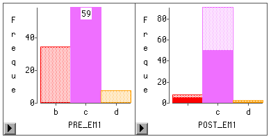
If you want to examine the data interactively, you may use the graphing function in SAS/Insight. In the bar chart when you click on any bar in the pre-test, the corresponding subjects will be highlighted in the post-test.

This Quicktime movie shows you how it works. The procedure of making an interactive bar chart is as the following:

• Import the data into a SAS library. Select Import from File and follow the on screen instruction. If the data have already been imported into a library, simply double-click the file icon. The dataset will be loaded into a temp library.

• Open Global/Analyze/Interactive Data Analysis.

• Select the dataset from the proper library.

• Select Histogram/Bar Chart from Analyse.

• Put one pre-test item and one post-test item into Y.

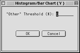
• Click on the button Method. Change "Other" Threshold to 0. Then SAS will show all values rather than collapsing some of them. Click OK to close it

• Click OK to plot the graph.

In addition, although a dependent t-test seems to be very straight-forward, you need to pay attention to some possible pitfalls:

First, a ceiling effect would obscure the finding of the true difference. A ceiling effect is that several respondents have mastered the subject matter before the treatment. For example, in the following table subject 1 achieved perfect scores in both pre-test and post-test. Although the difference between two tests is zero, it doesn't mean that your treatment is ineffective.

Obs	Pre-test	Post-test
1	10	10
2	5	8
3	6	9
4	7	10

To avoid the ceiling effect, you can simply exclude those "over-achievers.":

	if pretest = 10 then delete;

	proc means mean std n t prt; var diff;

Second, usually when you conduct a dependent t-test, you assume a directional hypothesis and apply a one-tailed test. In other words, you expect an improvement after the treatment rather than just a difference that can go either way. However, the default p-value of SAS is for a two-tailed test. Therefore, when the p-value is 0.10, which appears to be insignificant, the adjusted p-value for one-tailed test should be 0.05 (0.10/2)