Several assumptions for the data should be met in order to apply a valid regression model. Wonnacott and Winacott (1981) argued that if the assumptions of linearity, normality and independence are upheld, additional assumptions such as fixed values of X are not problematic. Berry & Feldman (1995) pointed out that most regression assumptions are concerned with residuals. This write-up will demonstrate how different assumptions of regression are examined.

Residuals have constant variance (homoescedasticity)

When the error term variance appears constant, the data are considered homoscedastic, otherwise, the data are said to be heteroscedastic. The SAS's syntax for checking residuals are as follows:

proc reg; model y = x1 x2; output out=two p=y_hat r=y_res; proc gplot data=two; plot y_res * y_hat;

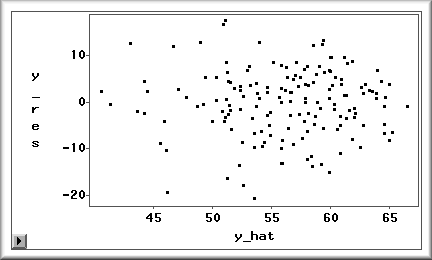
The outout is a plot of residuals versus predicted values. If the residuals variance is around zero, it implies that the assumption of homoscedasticity is not violated. If there is a high concentration of residuals above zero or below zero, the variance is not constant and thus a systematic error exists.

Independence of Residuals

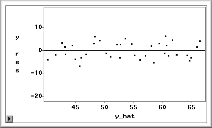
A regression model requires independence of error terms. Again, a residuals plot can be used to check this assumption. Random, patternless residuals imply independent errors. Even if the residuals are even distributed around zero and the assumption of constant variance of residuals is satisfied, the regression model is still questionable when there is a pattern in the residuals as shown in the following figure.

Normality of Residuals

It is important to note that for regression the normality test should be applied to the residuals rather than the raw scores. There isn't a general agreement of the best way to test normality. In SAS, there are four test statistics for detecting the presence of non-normality, namely, the Shapiro-Wilk (Shapiro & Wilk, 1965), the Kolmogorov-Smirnov test, Cramer von Mises test, and the Anderson-Darling test. According to the SAS manual, if the sample size is over 2000, the Kolmgorov test should be used. If the sample size is less than 2000, the Shapiro test is better. The null hypothesis of a normality test is that there is no significant departure from normality. When the p is more than .05, it fails to reject the null hypothesis and thus the assumption holds.

NCSS (NCSS Statistical Software, 2007) provides more normality tests in addition to the Shapiro test and the Kolmgorov test (see the following table). According to NCSS, the Shapiro and the Anderson Darling tests are the best. The Kolmogorov test is included just because of its historical popularity, but is bettered in almost every way by other tests.

However, some researchers argue that the Shapiro test was originally constructed to test a sample size carrying up to 50 subjects. To examine normality for a sample size between 51 to 1999, other tests such as Anderson-Darling, Martinez-Lglewicz, and D'Agostino tests are recommended.

Normality Test Section

Test Name	Test Value	Prob Level	10% Critical Value	5% Critical Value	Decision (5%)
Shapiro-Wilk W	0.937	0.21			Accept Normality
Anderson-Darling	0.443	0.29			Accept Normality
Martinez-Iglewicz	1.026		1.216	1.357	Accept Normality
Kolmogorov-Smirnov	0.148		0.176	0.192	Accept Normality
D'Agostino Skewness	1.037	0.299	1.645	1.960	Accept Normality
D'Agostino Kurtosis	-.786	0.432	1.645	1.960	Accept Normality
D'Agostino Omnibus	1.691	0.429	1.645	1.960	Accept Normality

Although many authors recommended using skewness and kurtosis for examining normality (Looney, 1995), Wilkinson (1999) argued that skewness and kurtosis often fail to detect distributional irregularities in the residuals. By this argument, the D'Agostino skewness and the D' Agostino Kurtosis test may be less useful.

Also, statistical tests depend on sample size, and as sample size increases, the tests often will reject innocuous assumptions. Most normality tests have small statistical power (probability of detecting nonnormal data) unless the sample size is large. If the null is rejected, the data are definitely non-normal. But if it fails to reject the null, the conclusion is uncertain. All you know is that there was not enough evidence to reject the normality assumption (NCSS Statistical Software, 2007). To rectify the sample size problem, Hair, Anderson, Tatham and Black (1992) suggested that in a small sample size it is safer to use both a normal probability plot and test statistics to ensure the normality. In SAS submitting the following command syntax returns both normal probability plot and test statistics.

 

proc univariate normal plot data=two; var y_res; histogram y_res/normal; QQplot y_res; run;

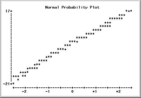
In a normal probability plot, the normal distribution is represented by a straight line angled at 45 degrees. The standard residuals are compared against the diagonal line to show the departure. If the residuals follow along the straight line, it means that the departure from normality is slight.
 

Residuals have mean as zero

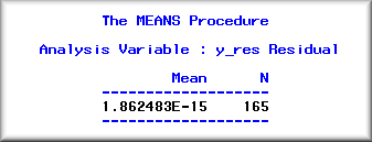
The above PROC UNIVARIATE statement returns the mean. One can also use PROC MEANS to get the same result. However, when the mean value carries many decimals, the SAS system will use E-notation. In the following example, the decimal point should shift 15 positions to the left, and thus the mean value is near zero (.000000000000001862483).

Linearity

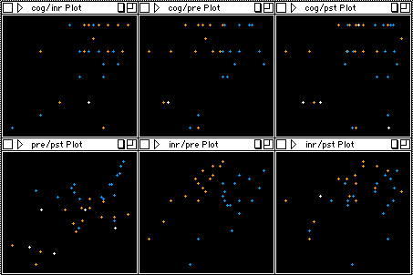
To examine the assumption of linearity, one can apply a scatterplot matrix showing all Xs against Y in a pairwise manner. However, this option is not available in SAS and SPSS's scatterplot matrix is not interactive. I recommend using an interactive scatterplot matrix, which is a feature of DataDesk. In a DataDesk's scatterplot matrix, one can assign colors to the data points for detecting clusters in different relationships. Take the following graphs as an example, the assumption of linearity seems to be violated because it appears that there are two clusters within the subjects. A linear fit to all data points is not the best fit.

Fox (1991) suggested that although it is useful to plot y against each x for the examination of linearity, these plots are inadequate because they only tell the partial relationship between y and each x, controlling for the other xs. Therefore, it is desirable to use residual plots against y. How to output residuals has been illustrated in the section of homoescedasticity. One can modify those methods by replacing the predicted values (Y hat) with the observed values (Y).

The absence of multicollinearity

Multicollinearity will cause the variances to be high. These inflated variances are quite detrimental to regression because some variables add very little or even no new and independent information to the model (Belsley, Kuh & Welsch, 1980). Although Schroeder, Sjoquist and Stephen (1986) asserted that there is no statistical test that can determine whether or not multicollinearity really is a problem, there are still several ways for detecting multicollinearity such as a matrix of bivariate correlation and the regression of each independent variable in the equation on all other independent variables (Berry and Feldman, 1985). Nonetheless, the former approach lacks sensitivity to multiple correlations while the latter cannot tell much about the influence of regressors to variances. A better approach is using the Variance Inflation Factor (VIF). The detail of detecting multicollinearity is in the write-up Multicollinearity, variance inflation factor, and orthogonalization.

 

Put all things together

It is more efficient to check all of the preceding issues at the same time. The following simple SAS macros was written for this purpose.
 

/* name = name of the data set dv = dependent variable, x1 = first independent variable, xlast = last independent variable */ %macro reg (name, dv, x1, xlast); proc reg data=&name; model &dv = &x1 - &xlast/vif; output out=two p=y_hat r=y_res; title "Check multicollinearity using VIF"; proc gplot data=two; plot y_res * y_hat; title "Check homoescedasticity and independence of residuals"; proc univariate normal plot data=two; var y_res; histogram y_res/normal; probplot y_res; QQplot y_res; title "Check the mean and normality of residuals"; proc gplot data=&name; plot &dv * (&x1 - &xlast); title "Check linearity"; run; %mend reg; /* To invoke the macros, enter the actual names of the data set, DV, fist IV, and the last IV in the following. */ %reg(name, dv, x1, xlast)

---

References

• Belsley, D. A., Kuh, E. & Welsch, R. E. (1980). Regression Diagnostics: Identifying influential data and sources of collinearity. John Wiley.

• Berry, W. D. & Feldman, S. (1985). Multiple regression in practice. London: Sage Publications.

• Fox, J. (1991). Regression diagnostics. Sage Publications.

• Looney, S. W. (1995). How to use tests for univariate normality to assess multivariate normality. American Statistician, 49, 64-70.

• NCSS Statistical Software. (2007). NCSS. [Computer Software] Kaysville, UT: Author.

• Schroeder, L. D., Sjoquist, D. L. & Stephan, P. E. (1986). Understanding regression analysis. Beverly Hills, CA: Sage Publications.

• Shapiro, S. S., & Wilk, M. B. (1965). An analysis of variance test for normality. Biometrika, 52, 591-611.

• Wilkinson, L, & Task Force on Statistical Inference. (1999). Statistical methods in psychology journals: Guidelines and explanations. American Psychologist, 54, 594-604.

• Wonnacott, T. H. & Wonnacott, R. J. (1981). Regression: A second course in statistics. Wiley.

Last updated: 2024

---

Navigation

Index

Simplified Navigation

Table of Contents

Search Engine

Contact