Resampling methods:
Concepts, Applications, and Justification

Keywords: Resampling, bootstrap, Jackknife, inference, counterfactual

Introduction

In recent years many emerging statistical analytical tools, such as exploratory data analysis (EDA), data visualization, robust procedures, and resampling methods, have been gaining attention among psychological and educational researchers. However, many researchers tend to embrace traditional statistical methods rather than experimenting with these new techniques, even though the data structure does not meet certain parametric assumptions. Three factors contribute to this conservative practice. First, newer methods are generally not included in statistics courses, and as a result, the concepts of these newer methods seem obscure to many people. Second, in the past most software developers devoted efforts to program statistical packages for conventional data analysis. Even if researchers are aware of these new techniques, the limited software availability hinders them from implementing them. Last, even with awareness of these concepts and access to software, some researchers hesitate to apply "marginal" procedures. Traditional procedures are perceived as founded on solid theoretical justification and empirical substantiation, while newer techniques face harsh criticisms and seem to be lacking theoretical support.

This article concentrates on one of the newer techniques, namely, resampling, and attempts to address the above issues. First, concepts of different types of resampling will be introduced with simple examples. Next, software applications for resampling are illustrated. Contrary to popular beliefs, many resampling tools are available in standard statistical applications such as SAS and SyStat. Resampling can also be performed in spreadsheet programs such as Excel. Last but not least, arguments for and against resampling are discussed. I propose that there should be more than one way to construe probabilistic inferences and that counterfactual reasoning is a viable means to justify use of resampling as an inferential tool.

What is resampling?

Classical parametric tests compare observed statistics to theoretical sampling distributions. Resampling is a revolutionary methodology because it departs from theoretical distributions. Rather, the inference is based upon repeated sampling within the same sample, and that is why this school is called resampling.

Resampling does not emerge without any context. Indeed, the resampling method is tied to the Monte Carlo simulation, in which researchers "make up" data and draw conclusions based on many possible scenarios (Lunneborg, 2000). The name "Monte Carlo" comes from an analogy to the gambling houses on the French Riviera. Many years ago, some gamblers studied how they could maximize their chances of winning by using simulations to check the probability of occurrence for each possible case. Today Monte Carlo simulations are widely used by statisticians to study the "behaviors" of different statistical procedures (e.g., Can the test still correctly reject the null hypothesis when the sample has unequal variances? Does the test have adequate statistical power?).

There are similarities and differences between resampling and Monte Carlo simulation. In resampling one could do all possible combinations, but it would be too time-consuming and computing-intensive. The alternative is Monte Carlo sampling, which restricts the resampling to a certain number. The fundamental difference between Monte Carlo simulation and resampling is that in the former data could be totally hypothetical, while in the latter the simulation must be based upon some real data.

Types of resampling

There are at least four major types of resampling. Although today they are unified under a common theme, it is important to note that these four techniques were developed by different people at different periods of time for different purposes.

• Randomization exact test: Also known as the permutation test, this test was developed by R. A. Fisher, the founder of classical statistical testing. However, in his later years Fisher lost interest in the permutation method because there were no computers in his days to automate such a laborious method.
  
  
• Cross-validation: Simple cross-validation was proposed by Kurtz (1948) as a remedy for the Rorschach test, a form of personality test which was criticized by psychometricians for its lack of common psychometric attributes such as data normality. Based on Kurtz's simple cross-validation, Mosier (1951) developed double cross-validation, which was later extended to multicross-validation by Krus and Fuller (1982).
  
  
• Jackknife: Also known as the Quenouille-Tukey Jackknife, this tool was invented by Maurice Quenouille (1949) and later developed by John W. Tukey (1958). As the father of EDA, John Tukey attempted to use Jackknife to explore how a model is influenced by subsets of observations when outliers are present. The name "Jackknife" was coined by Tukey to imply that the method is an all-purpose statistical tool.
  
  
• Bootstrap: This technique was invented by Bradley Efron (1979, 1981, 1982) and further developed by Efron and Tibshirani (1993). "Bootstrap" means that one available sample gives rise to many others by resampling (a concept reminiscent of pulling yourself up by your own bootstrap). While the original objective of cross-validation is to verify replicability of results and that of Jackknife is to detect outliers, Efron (1981, 1982) developed bootstrap with inferential purposes.

The principles of cross-validation, Jackknife, and bootstrap are very similar, but bootstrap overshadows the others for it is a more thorough procedure in the sense that it draws many more sub-samples than the others. Mooney and Duval (1993) suggested that Jackknife is of largely historical interest today. Through simulations Fan and Wang (1996) found that the bootstrap technique provides less biased and more consistent results than the Jackknife method does. Nevertheless, Jackknife is still useful in EDA for assessing how each sub-sample affects the model. Each technique will be explained in the following.

Randomization exact test

Although on many occasions the terms "randomization tests" and "permutation tests" are used interchangeably, the theories of randomization exact tests and permutation tests are slightly different (Edgington,1995). One fundamental difference is that exact tests exhaust all possible outcomes while resampling simulates a large number of possible outcomes. For this reason, some people treat exact tests and resampling as two different approaches. Randomization exact test is a test procedure in which data are randomly re-assigned so that an exact p-value is calculated based on the permutated data. Let's look at the following example (Table 1). Assume that in an experiment comparing Web-based and text-based instructional methods, subjects obtained the following scores:

Table 1 Original scores of two groups

Web-based		Text-based
Subject	Scores	Subject	Scores
Jody	99	Alex	87
Sandy	90	Andy	89
Barb	93	Candy	97
More subjects...	More scores...	More subjects...	More scores...

After the researcher has run a two-sample t-test, the test returns a t-value of 1.55. If the classical procedure is employed, the researcher can check this t_observed against the t_critical in the t-distribution to determine whether the group difference is significant. However, in resampling, instead of consulting a theoretical t-distribution, the researcher asks a "what-if" question: "It may just happen that Jody, the over-achiever, takes the Web-based version by chance, and Alex, the under-achiever, takes the text-based version by chance, too. What if their positions are swapped?" Then the researcher swaps the subjects and scores as shown in Table 2:

Table 2. Permutated scores of two groups

Web-based		Text-based
Subject	Scores	Subject	Scores
Alex	87	Jody	99
Sandy	90	Andy	89
Barb	93	Candy	97
More subjects...	More scores...	More subjects...	More scores...

In this swapping process the order of observations doesn't matter. The researcher doesn't care whether the order in one group is "Jody, Candy, Andy" (JCA) or "Candy, Jody, Andy" (CJA). For this reason, the term "permutation" is viewed as a misnomer by some mathematicians. In mathematics, there is a difference between combination and permutation. In the former the order of combinations doesn't matter, while in the latter different orders of combinations are considered different cases. To be specific, in permutation,

JCA <> JAC <> AJC <> ACJ <> CJA <> CAJ

Nevertheless, for now let's put aside this subtle difference and call the re-sample "the permutated data." Next, the researcher computes the permutated data and obtains another t-value of -0.64. If the researcher keeps swapping observations across the two groups, many more t-values will be returned. The purpose of this procedure is to artificially simulate "chance." Sometimes the t is large, but other times it is small. After exhausting every possibility, say 100, the inquirer can put these t-values together to plot an empirical distribution curve, which is built on the empirical sample data. When the t-value of 1.55 occurs only 5 times out of 100 times, the researcher can conclude that the exact p-value (the probability that this difference happens by chances alone) is .05. Since the experimenter compares the t_observed with the empirical t-distribution, the latter becomes the reference set. Other types of resampling are based on the same principle: repeated experiments within the same dataset.

Cross validation

In cross-validation, a sample is randomly divided into two or more subsets and test results are validated by comparing across sub-samples. Readers who are familiar with the classical test theory may find some degree of resemblance between spilt-half reliability and simple cross-validation. Indeed, the goal of both approaches, though in different contexts, is to find out whether the result is replicable or just a matter of random fluctuations. Cross validation could be classified into several categories, namely, simple cross-validation, double cross-validation, and multicross-validation.

Simple cross-validation. Take regression as an example. In the process of implementing a simple cross-validation, the first sub-sample is usually used for deriving the regression equation while another sub-sample is used for generating predicted scores from the first regression equation. Next, the cross-validity coefficient is computed by correlating the predicted scores and the observed scores on the outcome variable.

Double cross-validation. Double cross-validation is a step further than its simple counterpart. Take regression as an example again. In double cross-validation regression equations are generated in both sub-samples, and then both equations are used to generate predicted scores and cross-validity coefficients.

Multicross-validation. Multicross-validation is an extension of double cross-validation. In this form of cross-validation, double cross-validation procedures are repeated many times by randomly selecting sub-samples from the data set. In the context of regression analysis, beta weights computed in each sub-sample are used to predict the outcome variable in the corresponding sub-sample. Next, the observed and predicted scores of the outcome variable in each sub-sample are used to compute the cross validated coefficient.

Cross-validation suffers from the same weakness as spilt-half reliability when the sample size is small. By dividing the sample into two halves, each analysis is limited by a smaller number of observations. Ang (1998) argued that cross-validation is problematic because splitting an already small sample increases the risk that the beta weights are just artifacts of the sub-sample. Thus, Ang endorsed use of Jackknife, which will be discussed next.

Jackknife

Jackknife is a step beyond cross validation. In Jackknife, the same test is repeated by leaving one subject out each time. Thus, this technique is also called leave one out. This procedure is especially useful when the dispersion of the distribution is wide or extreme scores are present in the data set. In the following I will use a hypothetical regression model for illustration. In a research project test scores of multimedia knowledge and hypertext knowledge are used to predict test scores of internet knowledge (Table 3). However, the sample size (100) is relatively small and thus the stability of beta weights and R² is questionable.

Table 3. Small data set for regression analysis

Observation	IV1: Multimedia	IV2: Hypertext	DV: Internet
1	87	76	87
2	99	77	95
3	86	98	80
More observations...	More scores...	More subjects...	More scores...
50	99	87	99

As a remedy, the Jackknife technique is employed to assess the stability of the model. Regression analysis with this dataset could be repeated 50 times by omitting a different observation in each sub-sample. In each regression model, the pseudo-values of the beta weight and R² are computed by using the equation below:

Pseudo-value = N(theta prime of full sample) - (N-1)theta prime of sub-sample

whereas theta prime = beta weight or R²

In the example as shown in Table 4, after the first observation is deleted, the pseudo-values of beta weights of both predictors and the R² are computed by using the information obtained from the full sample and the sub-sample.

Table 4. Pseudo-values of beta weight and R²

	N=50	N=49
Beta weight of IV1	.16	.14	pseudo-values of IV1	50(.16)-49(.14)=1.14
Beta weight of IV2	.87	.77	pseudo-values of IV2	50(.87)-49(.77)=5.77
R2	.76	.80	pseudo-values of R2	50(.76)-49(.80)=-1.20

This calculation is repeated 50 times in order to obtain the pseudo-values of all sub-sample. Then, the Jackknifed coefficients are computed by averaging the pseudo-values (Table 5). The t_observed value can be obtained by dividing the Jackknifed coefficients by the standard error. Next, the t_observed can be compared with the t_critical to determine whether the Jackknifed coefficient is stable.

Table 5. Jackknifed coefficient

Observation deleted	pseudo-values of IV1	pseudo-values of IV2	pseudo-values of R2
1	1.14	5.77	1.20
2	1.68	4.87	2.11
3	2.19	3.77	1.87
4	2.11	2.34	3.01
5	1.09	1.09	3.11
More observations...	More pseudo-values...	More pseudo-values...	More pseudo-values...
Jackknifed coefficient	2.54	3.12	3.15

Bootstrap

Compared with the Jackknife technique, the resampling strategy of Bootstrap is more liberal. In bootstrap, the original sample is duplicated many times, and then this expanded sample is treated as a virtual population. Then samples are drawn from this population to verify the estimators. Obviously the "source" for resampling in bootstrap could be much larger than that in the other two. In addition, unlike cross validation and Jackknife, the bootstrap employs sampling with replacement. Further, in cross-validation and Jackknife, the n in the sub-sample is smaller than that in the original sample, but in bootstrap every resample has the same number of observations as the original sample. Thus, the bootstrap method has the advantage of modeling the impacts of the actual sample size (Fan & Wang, 1996).

Let's move away from regression for a bit and look at multiple-testing as an example (Table 6). In an experimental study there are two groups: a control group, consisting of 20 subjects, and a treatment group, consisting of 20 other subjects. Their subsequent use of various internet tools, such as email, FTP, Web browser, instant messaging, and online chat, are reported. For the ease of illustration, the dependent variables are defined as dichotomous (use or non use) rather than being expressed in some interval-scale. Since multiple effects are measured, the multiplicity of test hypotheses may lead to an inflation of Type I error. In this case, multiple test procedures in SAS (Westfall and Young, 1993), equivalent to multiple comparison procedures, can be employed. Nonetheless, the sample size is very small and it is doubtful whether any alleged effect derived from the treatment is really stable.

Table 6. Original data for multiple testing

Observations	Group	Email	FTP	Web	IM	Chat
1	Control	0	1	0	0	0
2	Control	0	1	0	1	1
3	Control	1	0	0	0	0
4	Control	0	0	0	0	0
5	Control	0	1	0	0	0
More observations...
21	Treatment	1	1	0	1	1
22	Treatment	1	0	1	1	1
23	Treatment	0	1	0	1	0
24	Treatment	1	1	1	0	0
25	Treatment	1	1	1	1	0
More observations...

In this case, this small size is duplicated 2000 times and then the virtual population is resampled 2000 times for analyzing the stability of the effects. In Table 7 the original p-values (raw) are compared side-by-side against the averaged p-values (bootstrap) obtained from the 2000 re-samples. Although based upon the original sample there is a treatment effect on the use of a Web browser (p=0.0286), the bootstrapped p-values tell a different story (p=.2210) and thus the alleged treatment effect on Web usage is considered unstable.

Table 7. Comparison of raw and bootstrap p-values

Variable	Contrast	Raw p-values	Bootstrap p-Values
Email	Treatment	0.0761	0.3160
FTP	Treatment	0.5451	0.9840
Web	Treatment	0.0286	0.2210
IM	Treatment	0.0761	0.3160
Chat	Treatment	0.5451	0.9840

Software for resampling

SAS

SAS (1997) can perform certain Jackknife and bootstrap analyses using macros programming. Nevertheless, bootstrap and permutation procedures have been built-in procedures in SAS (2002) since version 8. Figure 1 shows a simple example of employing bootstrap in multiple-testing. This example shows the "bootstrap" option, but "permutation" is also available in SAS. The "nsample" denotes the number of resamples, and in this case 2000 resamples are requested. The "seed" option allows the user to enter a different starting seed every time to ensure the randomness of the resampling process. The "pvals" option specifies the comparison of the original p-values and the bootstrapped p-values. The grouping variable is entered into the class statement while the outcome variables are entered in the test statement.

Figure 1. SAS code for bootstrapping

proc multtest bootstrap nsample=2000 seed=34268 pvals; class treatment; test ft(v1-v5); run;

SyStat

Although SyStat (2000) is not specifically developed for exact test, it has resampling functions to verify many conventional procedures such as ANOVA and regression. The syntax in SyStat for resampling is illustrated in Figure 4.

Figure 4. SyStat code for resampling

ESTIMATE / SAMPLE=BOOT(m,n) SIMPLE(m,n) JACK

The arguments m and n stand for the number of samples and the sample size of each sample. The parameter n is optional and defaults to the number of cases in the file. The BOOT option generates samples with replacement, SIMPLE generates samples without replacement, and JACK generates a jackknife set. For example, in a regression model one could compute the beta weights and the standard errors of the regressors, and then bootstrap the data to generate an empirical distribution of the coefficients. To evaluate the stability of the model, the observed coefficients and standard errors can be compared against their empirical counterparts. Figure 5 shows a typical example. It is important to note that this procedure is extremely computing-intensive. You should start from a smaller m (e.g., 200) and then increase the value of m gradually. It is not advisable to jump into 50,000 simulations in the first trial.

Figure 5. A bootstrap example in SyStat

USE dataset1 GLM MODEL Y=constant+X1+X2 SAVE BOOT / COEF ESTIMATE / SAMPLE=BOOT(500,30) OUTPUT TEXT1 USE dataset1 MODEL Y=constant+X1+X2 ESTIMATE

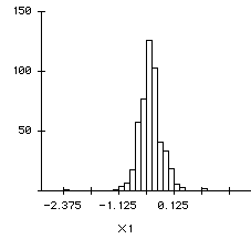
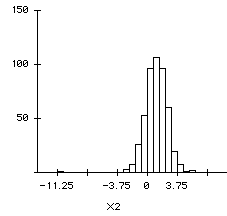
The histograms and the descriptive statistics of the empirical distribution of the coefficients are shown in Figures 6a, 6b and 7 (the graphs are created in Data-Desk based on the "bootstrap" dataset generated in SyStat):

Figure 6a Bootstrap estimator of X1's beta	Figure 6b Bootstrap estimator of X2's beta

Figure 7. Descriptive statistics of bootstrap estimators

Although the standard errors from the simulations are larger than the observed standard errors, both the observed beta weights of X1 (beta=-.04477, SE=-0.0461) and X2 (beta=.9334, SE=0.249) are very close to the mean of the distribution. The bootstrap result implies that the regression model is fairly stable.

 

Resampling Stats in Excel (RSE)

Resampling Stats (2001) provides resampling software in three formats: a standalone package, an Excel add-in module, and a Matlab plug-in module. For a long time some researchers (e.g., Willemain, 1994; Morris & Price, 1998) have been using spreadsheets for resampling because spreadsheet software packages, such as Lotus and Excel, are widely accessible. Because most users are familiar with a spreadsheet interface, this introduction will concentrate on the Excel version of Resampling Stats. Resampling Stats in Excel is a user-friendly and powerful resampling package. The only difficult part of using the package is to integrate it into Microsoft Excel. RSE requires the Analysis Pak and Analysis Visual Basic Extensions (VBX) to run. The user has to check both items in Tools/Add ins, close Excel, and then re-open Excel before the plug-in module can be used. There is no prompt for these steps and thus it may frustrates some users.

Resampling Stats in Excel conducts analysis through the Excel interface, which is already familiar to many users. The package is helpful not only in data analysis, but also in learning concepts of probability. Many statistical packages are like a "black-box": numbers in, numbers out. It is not unusual that many students and even faculty members are unable to explain the meaning of their analysis results. 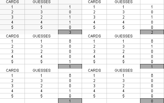The typical answer is: "This is what the computer software gives me." On the other hand, by analyzing data in RSE, the user can literally see the process step by step, as shown in the animation (Figure 2).

Figure 2. Permutation in RSE

For instance, in an example of testing Extra-Sensory Perception (ESP), the psychologist deals out five cards face down and asks the subject to guess which symbol is on the card. After a number of trials, a group of people gets 3 matches on the average. The questions are: Do they really possess the power of ESP? What is the probability of getting three matches by chance alone? To find out the likelihood of having this number of matches, the analyst can use the Shuffle function in RSE to simulate random guessing. Then he can use the Repeat and Score function to replicate the guessing process 1000 times. The simulated result is shown in Table 8. The frequency count of three matches out of 1000 times is 72; therefore, the probability is .072. If the experimenter considers a probability equal to or less than .05 significant, apparently these participants do not have ESP. RSE can solve many problems in this fashion.

Table 8. Repeat and score in RSE

Match	Counts (C)	Probability (C/1000)
0	415	.415
1	343	.343
2	162	.162
3	72	.072
4	7	.007
5	1	.001

StatXact

Cytel, Inc. (2000) has two modules for resampling: StatXact and LogXact. The former provides exacts tests for categorical data, while the latter provides test procedures for binary data. Use of StatXact is illustrated in the following with a real data set from a Web-based instruction project (Ohlund, Yu, DiGangi, & Jannasch-Pennell, 2001). Table 9 shows the number of participants who completed and did not complete the entire Web-based course, and the number of participants who used internet-based communication tools such as chat and email. The question is whether the use of internet communication makes a difference to the completion rate.

Table 9. Data set of Web-based instruction

	Both	Chat	Mail	None
Module Incomplete	0	7	5	54
Module complete	5	11	14	64

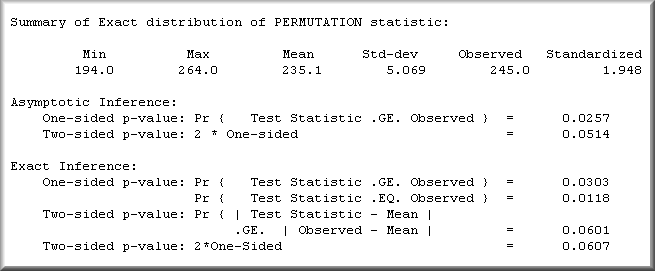
In this case Chi-square is not a valid test because some cells have a zero count. Thus, we turn to the permutation test and produce the output shown in Figure 3:

Figure 3. Exact Inference in StatXact

The asymptotic inference is based upon an approximation to the theoretical distribution. The exact inference is derived from the exact p-value. In both cases a statistically significant result is yielded. Therefore, we conclude that use of internet-based communication tools is related to the completion rate.

The above examples are by no means exhaustive; there are other resampling software applications on the market. The focus of this article is on standard software packages such as SAS, SyStat and Excel, but readers are encouraged to explore other viable tools.

Rationale of supporting resampling

Supporters of resampling have raised a number of reasons to justify the aforementioned techniques:

• Empirical: Classic procedures rely on theoretical distributions, which requires strong assumptions of both the sample and the population. But the inferential leap form the sample to the population may be problematic, especially when the population is ill-defined. If one is skeptical of the use of theoretical distributions, empirical-based resampling is a good alternative (Diaconis & Efron,1983; Peterson, 1991).
  
  
• Clarity: Conceptually speaking, resampling is clean and simple. Sophisticated mathematical background is not required to comprehend resampling. Thus, psychological and educational researchers, for example, can pay attention to the content of their research rather than worrying about which test procedure could reduce the family-wise error from 0.06 to 0.05 in multiple comparison. Further, because of its conceptual clarity, resampling-based statistics is a good learning tool. In a study where one group of students learned statistics through resampling and the other learned it in a conventional manner, the resampling group did much better in solving statistical problems than the conventional group (cited in Rudner & Shafer, 1992).
   
• Distribution: Classical procedures require distributional assumptions, which are usually met by a large sample size. When the sample size is small and does not conform to the parametric assumptions, resampling is recommended as a remedy (Diaconis & Efron,1983). However, Good (2000) stated that permutation tests are still subject to the Behrens-Fisher problem, in which estimation is problematic when population variances are unknown. To be specific, permutation tests still assume equal variances as what is required in classical tests.
   
• Non-random sample: Classical procedures require random sampling to validate the inference from a sample to a population. Edgington (1995) asserted that resampling is valid for any kind of data, including random and non-random data. Lunneborg (2000) suggested that although use of non-random samples in resampling may not lead to an inferential conclusion, at least subsampling of non-random samples can tell us more about the local description of the data and the stability of the result. Nonetheless, some researchers are still skeptical because a non-random sample may be a non-representative sample. If the sample that is used to generate the empirical sampling distribution does not reflect the characteristics of the population, then the validity of the inference is compromised. Philosopher of science Laudan (1977) emphasized that if a disadvantage is universal to all research traditions, then this disadvantage cannot be used to count against a particular research tradition. This notion is well-applied to the problem of non-random or non-representative samples. When the obtained sample is non-random or non-representative, classical procedures also have problems. Rodgers (1999) stated that all resampling techniques assume that the sample reflects the structure of the population. But classical procedures also make this assumption.
   
• Small sample size: Even if the data structure meets the parametric assumptions, a study with small sample size will be crippled by the low power level. Bootstrapping could treat a small sample as the virtual population to "generate" more observations.
   
• Large sample size: Usually resampling is a remedy for small sample size, however, the same technique can also be applied to the situation of overpowering, in which there are too many subjects. Given a very large sample size, one can reject virtually any null hypothesis. When the researcher obtains a large sample size, he/she could divide the sample into subsets, and then apply a simple or double cross-validation.
   
• Replications: Classical procedures do not inform researchers of how likely the results are to be replicated. Repeated experiments in resampling such as cross-validation and bootstrap can be used as internal replications (Thompson & Synder, 1997). Replications are essential to certain classical procedures such as multiple regression. Schumacker (1994) pointed out a common misconception that the best regression model is the one that includes all available significant predictors. The problem is that beta weights and R-square values are sample dependent due to the least square criterion being applied to a specific sample of data. It is important for the data analyst to cross-validate the result with other samples.

Criticisms of resampling

Despite these justifications, some methodologists are skeptical of resampling for the following reasons:

• Assumption: Stephen E. Fienberg mocked resampling by saying, "You're trying to get something for nothing. You use the same numbers over and over again until you get an answer that you can't get any other way. In order to do that, you have to assume something, and you may live to regret that hidden assumption later on" (cited in Peterson, 1991, p. 57). Every theory and procedure is built on certain assumptions and requires a leap of faith to some degree. Indeed, the classical statistics framework requires more assumptions than resampling does.
   
• Generalization: Some critics argued that resampling is based on one sample and therefore the generalization cannot go beyond that particular sample. One critic even went further to say, "I do wonder, though, why one would call this (resampling) inference?" (cited in Ludbrook & Dudley, 1998) Nevertheless, Fan and Wang (1996) stated that assessing the stability of test results is descriptive, not inferential, in nature.
   
• Bias and bad data: Bosch (2002) asserted that confidence intervals obtained by simple bootstrapping are always biased though the bias decreases with sample size. If the sample comes from a normal population, the bias in the size of the confidence interval is at least n/(n-1), where n is the sample size. Nevertheless, one can reduce the bias by more complex bootstrap procedures. Some critics challenged that when the collected data are biased, resampling would just repeat and magnify the same mistake. Rodgers (1999) admitted that the potential magnification of unusual features of the sample is certainly one of the major threats to the validity of the conclusion derived from resampling procedures. However, if one asserts that the data are biased, one must know the attributes of the underlying population. As a matter of fact, usually the population is infinite in size and unknown in distribution. Hence, it is difficult to judge whether the data are bad. Further, if the data were biased, classical procedures face the same problem as resampling. While replications in resampling could partially alleviate the problem, classical procedures do not provide any remedy.
   
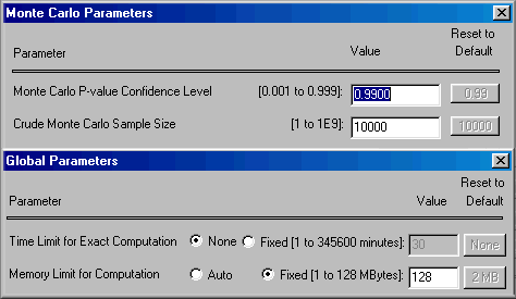
• Accuracy: Some critics question the accuracy of resampling estimates. If the researcher doesn't conduct enough experimental trials, resampling may be less accurate than conventional parametric methods. However, this doesn't seem to be a convincing argument because today's high-power computers are capable of running billions of simulations. For example, in StatXact, a software program for exact tests, the user could configure the resampling process to run with maximum RAM for 1000000000 samples with no time limit (Figure 8).
  
  Figure 8. Monte Carlo and Global parameters in StatXact

 

Resampling, probabilistic inference, and counterfactual reasoning

Can findings resulting from resampling be considered probabilistic inferences? The answer depends on the definition of probability. In the Fisherian tradition, probability is expressed in terms of relative long run frequency based upon a hypothetical and infinite distribution. Resampling is not considered a true probabilistic inference if the inferential process involves bridging between the sample and theoretical distributions. However, is this mode of inference just a convention? Why must the foundation of inference be theoretical distributions? Fisher asserted that theoretical distributions against which observed effects are tested have no objective reality, "being exclusively products of the statistician's imagination through the hypothesis which he has decided to test." (Fisher, 1956, p.81). In other words, he did not view distributions as outcomes of empirical replications that might actually be conducted (Yu & Ohlund, 2001). Lunneborg (2000) emphasized that resampling is a form of "realistic data analysis" (p.556) for he realized that the classical method of comparing observations to models may not be appropriate all the time. To be specific, how could we justify collecting empirical observations but using a non-empirical reference to make an inference? Are the t-, F-, Chi-square, and many other distributions just from a convention, or do they exist independently from the human world, like the Platonic reality? Whether such distributions are human convention or the Platonic metaphysical being, the basis of distributions remains the same: distributions are theoretical in nature, and are not yet empirically proven. As a matter of fact, there are alternative ways to construe probability. According to von Mises (1928/1957, 1964) and Reichenbach (1938), probability is the empirical and relative frequency based upon a finite sample. Other school of thoughts conceive probabilistic inferences in a logical or subjective fashion. Downplaying resampling by restricting the meaning of probabilistic inference to a certain school of probability may be counter-productive.

Rodgers (1999) argued that the ways in which we run our statistical analysis may be at least partially based on an "historical accident" (p.441); if Fisher's ANOVA had been invented 30 years later or computers had been available 30 years sooner, our statistical procedures would probably be less tied to theoretical distributions as what they are today. In my view, Fisher might not be opposed to resampling as a form of inference. Not only is this due to the fact that he is the inventor of the randomization test, but it is also because many of his methodologies, including design of experiment and randomization test, carry a common theme: counterfactual reasoning. A counterfactual inquirer tends to ask "what-if" questions. When X occurs and Y follows, the researcher could not jump to the conclusion that X causes Y. The relationship between X and Y could be "because of," "in spite of," or "regardless of." A counterfactual reasoner asks, "What would have happened to Y if X were not present?" In other words, the researcher does not base the judgment solely on the existing outcome, but also other potential outcomes. Thus, this reasoning model is also known as the potential outcome model.

When Rodgers argued that Fisher might have done ANOVA differently if computers were available, he was employing a form of counterfactual reasoning. One may argue that counterfactual reasoning is flawed because there is no way to verify a counterfactual claim; we cannot travel backward in time and give a computer to Fisher, nor can we bring Fisher to the 21^st century and observe what he would do with high-power computers. Actually, we always employ this form of reasoning. For example, if I drive 100 miles per hour on the highway, crash my car and injure myself, I would regret it and say, "If I didn't drive that fast, I would not have lost my vehicle or be in the hospital now." Nonetheless, no reasonable person would negate my statement by saying, "Your reasoning is flawed because you cannot verify the validity of your claim. You have already driven 100 miles per hour. You have wrecked your car and have hurt yourself. You cannot go backward in time and drive 50 miles per hour to learn what the alternative history is." Philosopher David Lewis (1973) believed that counterfactual logics carry certain merits and devoted tremendous endeavors to developing this form of reasoning. It is beyond the scope of this paper to discuss counterfactual philosophy; nevertheless, there are certain ways to verify a counterfactual claim. In my view, both resampling and classical statistics have a strong counterfactual element, though Fisher did not explicitly name the term.

In the classical Fisherian probability theory, the researcher rejects the null hypothesis because the observed results would be highly improbable compared to other possible outcomes (Howie, 2002). This inferential reasoning based upon comparison across different possible outcomes is counterfactual in essence. The randomization exact test utilizes the same sort of counterfactual logic. The researcher asks what other potential outcomes would result in all other possible scenarios, and the judgment is based on the comparison between the actual outcome and all possible outcomes. In short, in both procedures the researcher interprets probability in virtue of cases that have not occurred. It is interesting that this counterfactual logic is also noticeable in others of Fisher's inventions, such as his controlled randomization experimental design, in which subjects are randomly assigned to either the control group or the treatment group. The counterfactual aspect of controlled experimentation is that the control group gives information about how Y behaves when X is absent, while the treatment group tells the experimenter about how Y reacts when X is present. The latest probabilistic causal modeling promoted by Glymour and Pearl could be viewed as an extension of the counterfactual-based statistics and probability theories that originated from Fisher (Yu, 2001). Other resampling techniques, such as cross validation, Jackknife, and bootstrap, exhaust many more potential scenarios than the classical procedures. Thus, the conclusion derived from resampling should be qualified to be an inference in the sense of counterfactual logic, which is deeply embedded in the Fisherian tradition..

References

Ang, R. P. (1998). Use of Jackknife statistic to evaluate result replicability. Journal of General Psychology, 125, 218-228.

Bosch, P. V. (2002 May). Personal communication.

Cytel Corp. (2000). StatXact and LogXact. [On-line] Available: URL: http://www.cytel.com

Diaconis, P., and Efron, B. (1983). Computer-intensive methods in statistics. Scientific American, May, 116-130.

Edgington, E. S.(1995). Randomization tests. New York: M. Dekker.

Efron, B. (1979). Bootstrap methods: Another look at the jackknife. The Annals of Statistics, 7, 1-26.

Efron, B. (1981). Nonparametric estimates of standard error: The jackknife, the bootstrap and other methods. Biometrika, 63, 589-599.

Efron, B. (1982). The jackknife, the bootstrap, and other resampling plans. Society of Industrial and Applied Mathematics CBMS-NSF Monographs, 38.

Efron, B., & Tibshirani, R. J. (1993). An introduction to the bootstrap. New York: Chapman & Hall.

Fan, X., & Wang, L. (1996). Comparability of jackknife and bootstrap results: An investigation for a case of canonical correlation analysis. Journal of Experimental Education, 64, 173-189.

Fisher, R. A. (1956). Statistical methods and scientific inference. Edinburgh: Oliver and Boyd.

Good, P. (2000). Permutation Tests: A Practical Guide to Resampling Methods for Testing Hypotheses. New York: Springer-Verlag.

Howie, D. (2002). Interpreting probability: Controversies and developments in the early twentieth century. Cambridge, UK: Cambridge University Press.

Krus, D. J., & Fuller, E. A. (1982). Computer-assisted multicross-validation in regression analysis. Educational and Psychological Measurement, 42, 187-193.

Krurtz, A. K. (1948). A research test of Rorschach test. Personnel Psychology, 1, 41-53.

Laudan, L. (1977). Progress and its problem: Towards a theory of scientific growth. Berkeley, CA: University of California Press.

Lewis, D. (1973). Counterfactuals. Oxford: Blackwell.

Ludbrook, J. & Dudley, H. (1998). Why permutation tests are superior to t and F tests in biomedical research. American Statistician, 52, 127-132.

Lunneborg, C. E. (2000). Data analysis by resampling: Concepts and Applications. Pacific Grove, CA: Duxbury.

Mooney, C. Z. & Duval, R. D. (1993). Bootstrapping: A nonparametric approach to statistical inference. Newbury Park, CA: Sage Publications.

Morris, R. L., & Price, B. A. (1998). A spreadsheet approach to teaching resampling. Journal of Education for Business, 73, 358-363.

Mosier, C. I. (1951). Problems and designs of cross-validation. Educational and Psychological Measurement, 11, 5-11.

Ohlund, B., Yu, C.H., DiGangi, S., & Jannasch-Pennell, A. (2001). Impact of asynchronous and synchronous Internet-based communication on collaboration and performance among K-12 teachers. Journal of Educational Computing Research, 23, 435-450.

Peterson, I. (July 27, 1991). Pick a sample. Science News, 140, 56-58.

Quenouille, M. (1949). Approximate tests of correlation in time series. Journal of the Royal Statistical Society, Soc. Series B, 11, 18-84.

Reichenbach, H. (1938). Experience and prediction: An analysis of the foundations and the structure of knowledge. Chicago, IL.: The University of Chicago Press.

Resampling Stat. [Computer software] (2001). Resampling Stat for Excel 2.0. Arlington, VA: Resampling Stat [On-line] Available: http://resample.com.

Rodgers, J. L. (1999). The bootstrap, the jackknife, and the randomization test: A sample taxonomy. Multivariate behavioral research, 34, 441-456.

Rudner, L. M. & Shafer, M. Morello (1992). Resampling: a marriage of computers and statistics. Practical Assessment, Research & Evaluation, 3(5). [On-line] Available: http://edresearch.org/pare/getvn.asp?v=3&n=5

SAS [Computer software] (1997). Subsetting and resampling in SAS. SAS Institute. [On-line] Available: http://www.utexas.edu/acits/docs/stat56.html.

SAS [Computer software] (2002). SAS version 8. Cary, NC: SAS Institute. [On-line] Available: http://www.sas.com

Schumacker, R. E. (1994 April). A comparison of the Mallows' CP and principal component criteria for best model selection in multiple regression. Paper presented at the American Educational Research Association. New Orleans, LA.

Simon, J. L. (1998). Resampling: The new statistics. [On-line] Available: http://www.resample.com/book/contents.htm

SyStat [Computer software] (2000). SyStat Version 10. Richmond, CA: SyStat Inc. [On-line] Available: http://www.systat.com/

Thompson, B., & Snyder, P. A. (1997). Statistical significance testing practices in the Journal of Experimental Education. Journal of Experimental Education, 66, 75-83.

Tukey, J. W. (1958). Bias and confidence in not quite large samples. Annals of Mathematical Statistics, 29, 614.

von Mises, R. (1928/1957). Probability, statistics, and truth. London: The Macmillan Company.

von Mises, R. (1964). Mathematical theory of probability and statistics. New York: Academic Press.

Westfall, P.H. and Young, S.S. (1993). Resampling-based multiple testing: Examples and methods for p-value adjustment. New York: John Wiley & Sons, Inc.

Williemain, T. R. (1994). Bootstrap on a shoestring: Resampling using spreadsheets. American Statistician, 48, 40-42.

Yu, C. H. (2001). Philosophical foundations of causality in statistical modeling. Research Method Forum, 6. [On-line] Available URL: http://www.aom.pace.edu/rmd/2001forum.html

Yu, C. H., & Ohlund, B. (2001 ). Mathematical Reality: An inquiry into the existence of theoretical distributions and its implication to psychological Researchers. Paper presented at the Annual Meeting of Arizona Educational Researcher Organization, Tempe, AZ. (ERIC Document Reproduction Service No. ED 458 236)

Go up to the main menu

Navigation Home Other courses Search Engine

Contact me