Collinearity
First, let's look at multicollinearity from a
conventional viewpoint.
The absence of multi-collinearity is essential to a multiple regression
model.
In regression when several predictors (regressors) are highly
correlated,
this problem is called multi-collinearity or collinearity. When things
are related,
we say they are linearly dependent on each other
because you can nicely fit a straight regression line to pass through
many data points of those variables. Collinearity simply means co-dependence.
Why is co-dependence of predictors detrimental?
Think about a couple in a jury. If two persons who are husband and wife
are both members of a jury, the judge
should dismiss either one of them, because their decisions may
dependent on each other and thus bias the outcome.
Collinearity is problematic when one's purpose is
explanation rather than mere prediction (Vaughan & Berry,
2005). Collinearity makes it more difficult to achieve significance of
the collinear parameters. But if such estimates are statistically
significant, they are as
reliable as any other variables in a model. And even if they are not
significant,, the sum
of the coefficient is likely to be reliable. In this case, increasing
the sample size is a viable remedy for collinearity when prediction
instead of explanation
is the goal (Leahy, 2001). However, if the goal is explanation,
improving measures other than increasing the sample size are needed.
VIF
Understanding multi-collinearity should go hand in
hand with understanding variation inflation. Variation inflation is the
consequence of multi-collinearity. We may say multi-collinearity is the
symptom while variance inflation is the disease. In a regression model
we expect a high variance explained (R-square). The higher the variance
explained is, the better the model is. However, if collinearity exists,
probably the variance, standard error, parameter estimates are all
inflated. In other words, the high variance is not a result of good
independent predictors, but a mis-specified model that carries mutually
dependent and thus redundant predictors! Variance inflation factor
(VIF) is common way for detecting multicollinearity. In SAS you can
obtain VIF in the following ways:
PROC REG; MODEL Y = X1
X2 X3 X4
/VIF
The VIF option in the regression procedure can be interpreted in the
following ways:
- Mathematically speaking: VIF =
1/(1-R-square)
- Procedurally speaking: The SAS
system put each independent variables as the dependent variable e.g.
X1 = X2
X3 X4
X2 = X1 X3
X4
X3 = X1 X2
X4
Each model will return an R-square and VIF. We can
decide to throw out which variable by examining the size of VIF. There
is no consensus regarding the acceptable level of the VIF. A general
rule is that the VIF should not exceed 10 (Belsley, Kuh, & Welsch,
1980; Vittinghoff, Glidden, Shiboski, & McCulloch, 2012). However,
some authors prefer more conservative thresholds, ranging from .25
(James, Witten, Hastie, & Tibshirani, 2021; Johnston, Jones, &
Manleto, 2018) to 5 (Menard, 2001).
- Graphically speaking: In a Venn
Diagram, VIF is shown by many overlapping circles. In the following
figure, the circle at the center represents the outcome variable and
all surrounding ones represent the
independent variables. The superimposing area denotes the variance
explained. When there are too many variables, it is likely that Y is
almost entirely covered by many inter-related Xs.
The variance explained is very high but this model is over-specified
and thus useless.

For example, a student asked me what variables are related to school
performance. In other words, he wants to know how he could improve his
grade. I told him that my fifty-variable regression model could predict
almost 100 percent of class performance. So, I told him to do the
following: study long hours, earn more money, marry a good wife, buy a
reliable car, watch less TV, browse more often on the Web, exercise
more often, attend church more often, pray more often, go to fewer
movies, play fewer video games, cut your hair more often, drink more
milk and coffee...etc. Needless to say, this "overspecified" advice
derived from a overspecified regression model with collinear predictors
and artificially inflated variance is totally useless.
In research it is not enough to have a high number if
you don't know what it means. With too many independent variables, you
don't know which variables were adequate predictors and which were
noise. A sharpshooter might fire twice and hit a target, a poor shooter
can use a machine gun to blow away a target with 100 bullets. Both hit
the target, but the sharpshooter knows why it happened.
A frequently used remedy for too many variables is
stepwise regression. But I don't recommend this approach. Instead,
"Maximum R-square," "Root mean square error," and "Mallow's CP" are
considered better alternatives. The detail will be discussed in the
section "stepwise regression."
Ridge regression
When multicollinearity occurs, the variances are
large and thus far from the true value. Ridge regression is an
effective counter measure because it allows better interpretation of
the regression coefficients by imposing some bias on the regression
coefficients and shrinking their variances (Morris, 1982; Pagel
& Lunneberg, 1985; Nooney & Duval, 1993).
Let's use factor analysis as a metaphor to understand
ridge regression. If a researcher develops a survey with a hundred
items, he will not use a hundred variables in a regression model. He
measures the same constructs several times by different questions for
reliability estimation. In this case, he will conduct factor analysis
or principal component to collapse those items into a few latent
constructs. These few constructs will be served as regressors instead.
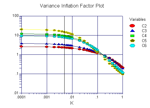
By the same token, ridge regression replaces inter-correlated
predictors with principal components. The following figure shows a
portion of the ridge regression output in NCSS (NCSS Statistical
Software, 2007).

The following is an example of performing ridge
regression in SAS: