Polynomial regression
| Not all
regression models are linear. In some situations the relationship among
variables may be non-linear.
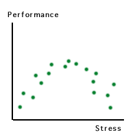
A classic example is stress-performance relationship. Initially
pressure could lead to better efficiency.
But if the stress is too intense, performance will decrease due to
physical or mental break down.
|
 |

|
Another
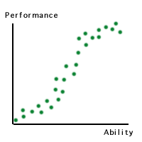
classic example is the relationship between performance and ability.
Contrary to popular belief, increasing ability in a discipline or a
specific task does not lead to a linear increase in performance. Many
teachers are frustrated with the phenomenon that many low achievers do
not show improvement in test scores despite tremendous efforts
contributed by both teachers and students. It is because low-ability
learners do not have the required skills to perform even the basic
function. Once they master the basic skills, their performance gain
would be proportional to their ability gain. The curve hits an
inflection point and turn virtually flat again when their ability are
matured. For example, the score difference in a writing test between a
master and a Ph.D. may be minimal. The technical term for this S-shaped
curve is ogive.
|
In curvilinear cases, polynomial regressions, which involve quadratic,
cubic, or quartic terms, should be implemented.
The equations of polynomial regressions are listed in the following:
| Quadratic: |
Y = A + B1X + B2X2
|
| Cubic: |
Y = A + B1X + B2X2
+ B3X3
|
| Quartic: |
Y = A + B1X + B2X2
+ B3X3 + B4X4
|
Which term should be used depends on the number of "turns" (inflection
points) on the non-linear curve. In case 1 there is only one turn on
the curve and a quadratic term should be used. In case 2 there are two
inflection points and thus a cubic term should be applied.
Gram-Schmidt method
Can you smell the smoke of multi-collinearity? Are
the quadratic, cubic, quartic and the original variables highly
correlated?
Yes, of course. The first three are derived from raising power of the
original variable.
To avoid the problem of multi-collinearity, again you should
"orthogonalize" the vectors. Again, centered-score regression can be
used for partial orthogonalization (Neter, Wasserman, & Kutner,
1990). Nonetheless, the Gram-Schmidt method, which
is a full orthogonalization approach, is considered a better approach.
The explanation of Gram-Schmidt method is beyond the scope of this
tutorial. Please consult the book by Saville and Wood (1991) for
detail. Nevertheless, the concept of orthogonalization remains the same
here.
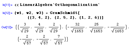
One of the easiest way to perform Gram-Schmidt
orthogonalization is using Mathemetica. It takes only two lines of
command syntax to transform the vectors (see the following panel). The
first step is to load the Orthogonalization function. It is important
to note that the symbols before and after the phrase
"Orthogonalization" are an accent mark(`) (the key is located at the
upper left corner of the keyboard), not quotation mark ('). The second
step is to output the original vectors to new orthogonal vectors.

PROC ORTHOREG
Another way to orthogonalize the vectors in the
regression is to employ PROC ORTHOREG in SAS. This procedure is
specifically developed for ill-conditioned data and polynomial model.
The orthogonalization method here is Gentleman-Givens
transformations. The following example is a labor statistics
dataset in the SAS manual. Price level, GNP, unemployment rate, size of
armed forces, population, and year are used to predict employment rate.
The raw variables are strongly correlated and it is believed that the
regression model is a quadratic model. Because collinearity became a
threat to the stability of the model, PROC ORTHOREG instead of PROC REG
or PROC GLM is used in the estimation.
	proc orthoreg; model Employment =
	Prices Prices*Prices
	GNP GNP*GNP
	Jobless Jobless*Jobless
	Military Military*Military
	PopSize PopSize*PopSize
	Year Year*Year;
Navigation
Index
Simplified Navigation
Table of Contents
Search Engine
Contact