However, if the Likert scale starts from 0, such as the ATUST, the above formula will not work. For example, if the value in a negative statement is "0," the new value will be "8" (8 - 0 = 8)
after the conversion. In this case one-dimensional array can be used to convert the scale:
In the preceding program, an array with eleven slots are created. All items which carry negative statements are put into the array. Next, a do loop tells SAS to make the conversion eleven times.
Within the do loop, if-then-else logical branching is used to reverse the scale for those eleven items.
 One may argue that when a high Cronbach Alpha indicates a high degree of internal consistency, the test or the survey must be uni-dimensional rather than multi-dimensional. Thus, there is no need
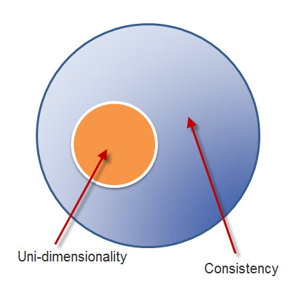
to further investigate its subscales. This is a common misconception. Actually consistency and dimensionality must be assessed separately. The relationship between inconsistency and uni-dimensionality is illustrated in the figure on the left. Uni-dimensionalityis a subset of consistency. If a test is uni-dimensional, then it will show internal consistency. But if a test is internally consistent, it does not necessarily entail one construct (Gardner, 1995; 1996). Internal consistency is a form of reliability while dimensionality is associated with construct validity. Reliability is a necessary, but not a sufficient condition, for validity. This logic works like this: If I am a man, I must be a human. But if I am a human, I may not be a man (could be a woman). The logical fallacy that "if A then B; if B then A" is termed as "affirming the consequent" (Kelly, 1998). This fallacy often happens in the misinterpretation of Cronbach Alpha.
One may argue that when a high Cronbach Alpha indicates a high degree of internal consistency, the test or the survey must be uni-dimensional rather than multi-dimensional. Thus, there is no need
to further investigate its subscales. This is a common misconception. Actually consistency and dimensionality must be assessed separately. The relationship between inconsistency and uni-dimensionality is illustrated in the figure on the left. Uni-dimensionalityis a subset of consistency. If a test is uni-dimensional, then it will show internal consistency. But if a test is internally consistent, it does not necessarily entail one construct (Gardner, 1995; 1996). Internal consistency is a form of reliability while dimensionality is associated with construct validity. Reliability is a necessary, but not a sufficient condition, for validity. This logic works like this: If I am a man, I must be a human. But if I am a human, I may not be a man (could be a woman). The logical fallacy that "if A then B; if B then A" is termed as "affirming the consequent" (Kelly, 1998). This fallacy often happens in the misinterpretation of Cronbach Alpha.
Gardner (1995) used a nine-item scale as an example to explain why a high Alpha does not necessarily indicate one dimension: Cronbach Alpha is a measure of common variance shared by test items. The Cronbach Alpha could be high when each test item shares variance with at least some other items; it does not have to share variance with all other items.
Different possible scenarios are illustrated in the following figures. As mentioned before, Cronbach Alpha can be calculated based upon item correlation. When the correlation coefficient is squared, it becomes the strength of determination, which indicates variance explained. Variance explained is often visualized by sets. When two sets are intersected, the overlapped portion denotes common variance. The non-overlapped portion indicates independent information.
 In the first scenerio, all nine sets have no overlapped area, and thus all nine items share no common variance. They are neither internally consistent nor uni-dimensional. In this situation, interpreting a low Alpha as the absence of uni-dimensionality is correct.
 The second scenario is exactly opposite to the first one. It shows the presence of a high degree of internal consistency and uni-dimensionality because all items share common variance with each other. Interpreting a high alpha as an indication of the presence of one single construct could be accepted.
 Unlike the above two situations, the last scenario is misleading. In Figure 6c, several items share variance with some others. In other words, subscales exist inside the instrument even though the Alpha is high and the instrument is internally consistent. Interpreting a high Alpha as a sign of uni-dimensionality is problematic.
A real life example is found in a sociological research concerning cognitive and affective attitudes toward sex. Originally, the cognitive scale and the affective scale are treated as two scales. Cronbach Alphas of the two scales are high (cognitive = .87, affective = .85) and thus it gave an illusion that the two scales represent two constructs only. However, factor analysis indicated that indeed there are two subscales in each scale. After spliting the two scales into four, Alphas were improved (see the following table).
|
Scales
|
Alphas
|
Sub-scales
|
Alphas
|
|
Cognitive attitude toward sex
|
.87
|
Cognitive attitude toward sexual behaviors
|
.92
|
|
Cognitive attitude toward using condoms
|
.95
|
|
Affective attitude toward sex
|
.85
|
Affective attitude toward sexual behaviors
|
.91
|
|
Affective attitude toward using condoms
|
.88
|
Verify the number of factors
You can run a factor analysis to verify the numnber of factors (subscales) using this SAS code: proc factor
method=ml priors=smc scree; var a1-a31;
"ML" stands for maximum likelihood and "SMC" means squared multiple correlation. If these options are omitted, by default SAS
uses Principal Component Analysis (PCA). SAS syntaxes are misleading because PCA
is under "proc factor," but indeed PCA and factor analysis are conceptually
different. PCA is just for data reduction, in which multiple variables are
reduced to one or a few manageable components. But the purpose of factor
analysis is to classify items or variables according to constructs.
The original graphical output from SAS is too big to fit in a page and thus the above graph is a truncated version. The first two factors and variable 21 to variable 31 are not shown on the scree plot.
There are several ways to determine how many factors should be retained in a model. Scree plot and Kasier's criterion are two common ways. In a scree plot the number of factors is
plotted against the eigenavlue. The cutoff is at the inflection point, where the slope has a sharp change. In this example the inflection point is indicated by red
arrows. In Kasier's criterion, the cutoff is that "eigenavlue is equal to or greater than 1." In this example, the Kasier's criterion is depicted by a blue
line.
Based upon the scree plot and the Kasier's criterion, seven subscales could be extracted from the data.
Correlation matrix
Even if there are seven subscales in the instrument, their independence remains a question. The evaluator should collapse the items into seven subscales according to the instrument manual, and then
check the inter-correlation of the subscales. In addition, the Cronbach coefficient Alpha of each subscale should be checked, too. The SAS code is as the following:
aware = sum(of a3 a12 a21 a23 a30);
info = sum(of a6 a14 a15 a26 a35);
person = sum(of a7 a13 a17 a28 a33);
manage = sum(of a4 a8 a16 a25 a34);
conseq = sum(of a1 a11 a19 a24 a32);
colla = sum(of a5 a10 a18 a27 a29);
refocus = sum(of a2 a9 a20 a22 a31);
proc corr;
	var aware info person manage conseq colla refocus;
proc corr alpha nomiss;
	var a1-a35;
proc corr alpha nomiss;
	var a3 a12 a21 a23 a30;
proc corr alpha nomiss;
	var a6 a14 a15 a26 a35;
proc corr alpha nomiss;
	var a7 a13 a17 a28 a33;
proc corr alpha nomiss;
	var a4 a8 a16 a25 a34;
proc corr alpha nomiss;
	var a1 a11 a19 a24 a32;
proc corr alpha nomiss;
	var a5 a10 a18 a27 a29;
proc corr alpha nomiss;
	var a2 a9 a20 a22 a31;
|
It is important to note that a negative correlation is not a problem in data analysis. For example, if the instrument has a subscale measuring "individualism" and another subscale assessing
"collaboration," it is expected that they should be opposite to each other conceptually and their relationship should be inverse.
On the other hand, a positive relationship is a problem because the concepts measured by the subscales are not distinct.
In this example, only two subcales, "management" and "collaboration" are independent and sustain an acceptable Cronbach coefficient Alpha.
Please keep in mind that PROC FACTOR in SAS is mainly for exploratory factor analysis. But some researchers suggest that exploratory tetrad analysis (ETA) outperforms EFA in removing impure indicators that do not belong to the target factor (Glymour et al., 1987). Unlike conventional factor analysis, TETRAD explores different path combinations (possible relationships between observed items and latent constructs) by path searching. To learn how to use TETRAD for path searching, please view this short movie clip (This tutorial was created with the help of Michelle Miller).
For confirmatory factor analysis (CFA), PROC CALIS in SAS or AMOS in SPSS should be employed. Nevertheless, in recent years some researchers suggested that the Rasch model is a superior method to CFA in terms of confirming a factor structure (Waught & Chapman, 2005).
References
Gardner, P. L. (1995). Measuring attitudes to science: Unidimensionality and internal consistency revisited. Research in Science Education, 25, 283-9.
Gardner, P. L. (1996). The dimensionality of attitude scales: A widely misunderstood idea. International Journal of Science Education, 18, 913-9.
Glymour, C., Scheines, R., Spirtes, P., & Kelly, K. (1987). Discovering causal structure. Orlando, FL: Academic Press.
Kelley, D. (1998). The art of reasoning (3rd ed.). New York: W. W. Norton & Company.
Waugh, R. F., & Chapman, E. S. (2005). An analysis of dimensionality using factor analysis (True-score theory) and Rasch Measurement: What is the difference? Which method is better? Journal of Applied Measurement, 6, 80-99.
Navigation

Press this icon to contact Dr. Yu via various channels